Overview
This project explores 2D convolution, finite-difference gradients, derivatives of Gaussians (DoG), unsharp masking, hybrid images, and multi‑resolution blending. I implement convolution from scratch, analyze edge detection with/without Gaussian smoothing, create hybrid images following Oliva–Torralba–Schyns, and reproduce the classic oraple blend using Gaussian/Laplacian stacks and mask pyramids.
Table of Contents
Part 1.1 — Convolutions from Scratch
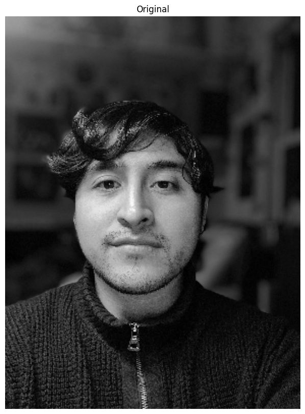
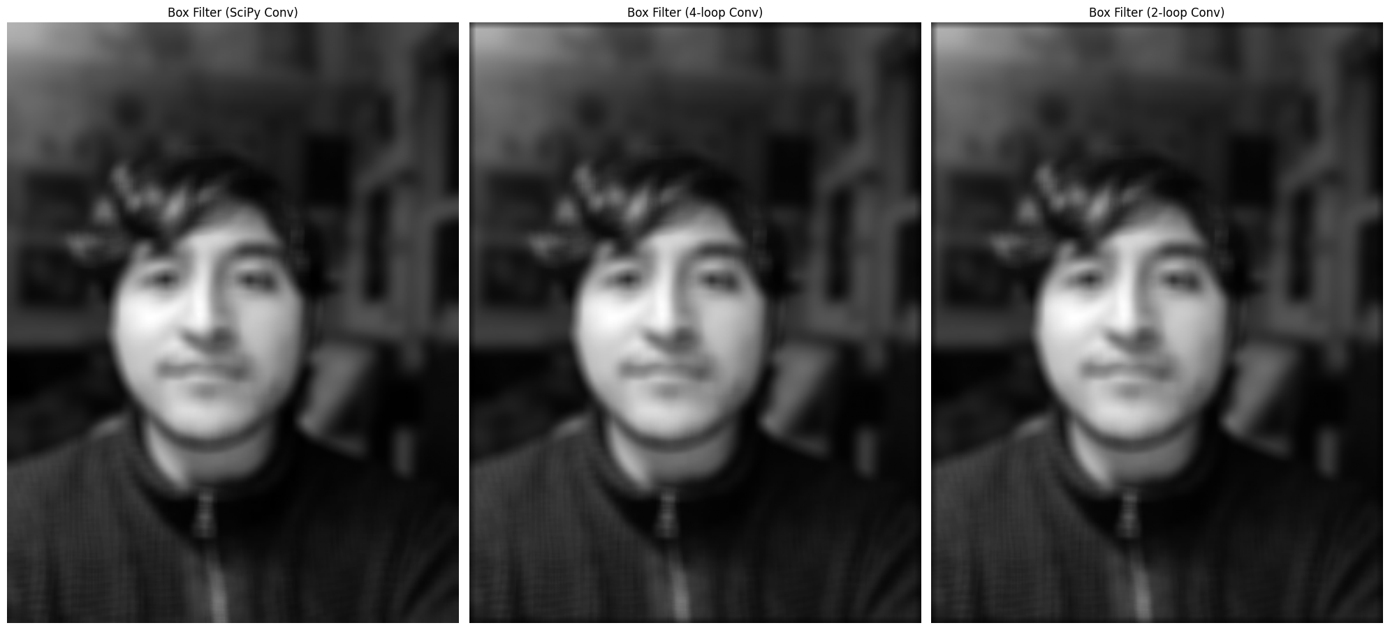
I implemented 2D convolution with explicit loops (4‑loop baseline, then 2‑loop optimization) and matched SciPy’s convolve2d with zero padding. Below I show the self‑portrait and the 9×9 box‑filtered result.
Code — Part 1.1 Convolution from Scratch
    def convolution_4(img, kernel):
      kernel = np.flip(kernel, axis=(0,1))

      img_h, img_w = img.shape
      ker_h, ker_w = kernel.shape

      pad_h, pad_w = ker_h // 2, ker_w //2
      pad_img = np.pad(img, ((pad_h, pad_h),(pad_w, pad_w)), mode="constant")
      pad_img_h, pad_img_w = pad_img.shape

      conv_img = np.zeros_like(img, dtype=np.float64)
      for i in range(img_h):
          for j in range(img_w):
              for k in range(ker_h):
                  for l in range(ker_w):
                       conv_img[i,j] += pad_img[i+k, j+l] * kernel[k,l]
      return conv_img


    def convolution_2(img, kernel):
      kernel = np.flip(kernel, axis=(0,1))

      img_h, img_w = img.shape
      ker_h, ker_w = kernel.shape

      pad_h, pad_w = ker_h // 2, ker_w //2
      pad_img = np.pad(img, ((pad_h, pad_h),(pad_w, pad_w)), mode="constant")
      pad_img_h, pad_img_w = pad_img.shape

      conv_img = np.zeros_like(img, dtype=np.float64)
      for i in range(img_h):
          for j in range(img_w):
              conv_img[i,j] = np.sum(pad_img[i:i+ker_h, j:j+ker_w] * kernel)
      return conv_img
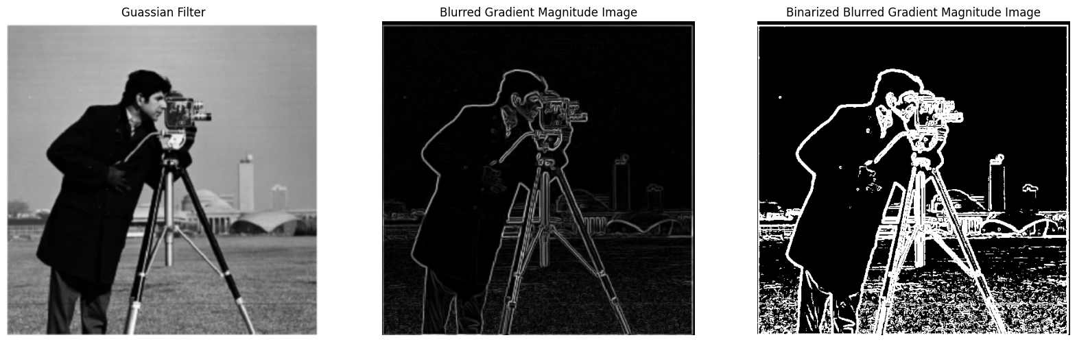
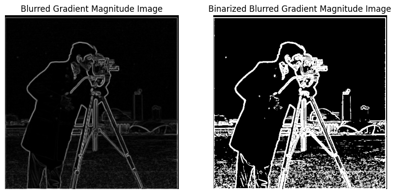
Part 1.2 — Gradient Magnitude
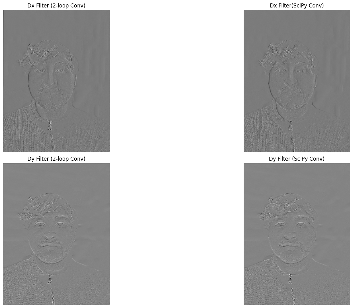
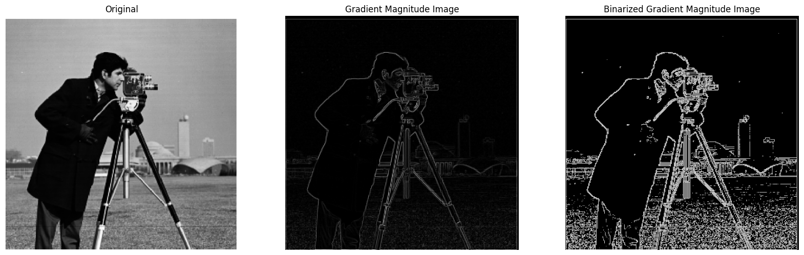
I computed partial derivatives using finite difference operators Dx=[-1,1] and Dy=[-1;1], formed the gradient magnitude, and thresholded to get a binarized edge map.
Code — Part 1.2 Finite Differences & Gradient Magnitude
    def gradient_magnitude_img(Dx_img, Dy_img):
      grad_mag_img = np.sqrt(Dx_img**2 + Dy_img**2)
      return grad_mag_img / grad_mag_img.max()

    img = np.array(Image.open("cameraman.png").convert("L"))
    Dx = np.array([[-1, 1]], dtype=np.float64)
    Dy = np.array([[-1], [1]], dtype=np.float64)

    Dx_img = convolve2d(img, Dx, mode="same", boundary="symm")
    Dy_img = convolve2d(img, Dy, mode="same", boundary="symm")
    grad_mag_img = gradient_magnitude_img(Dx_img, Dy_img)

    grad_mag_img_binarized = grad_mag_img.copy()
    grad_mag_img_binarized[grad_mag_img_binarized < 0.07] = 0
    grad_mag_img_binarized[grad_mag_img_binarized >= 0.07] = 1
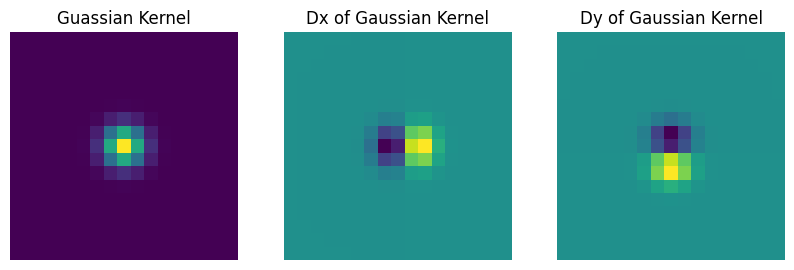
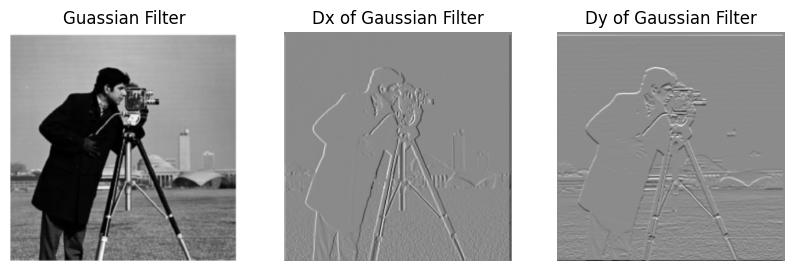
Part 1.3 — Derivative of Gaussian (DoG)
I first smoothed with a Gaussian then applied finite differences; next I created DoG filters by convolving the Gaussian kernel with Dx, Dy to achieve the same result with a single convolution. The DoG pipeline suppresses noise while preserving edges.
Code — Part 1.3 Gaussian & DoG
    gaussian_kernel_1D = getGaussianKernel(17, 1)
    gaussian_kernel_2D = gaussian_kernel_1D @ gaussian_kernel_1D.T

    Dx = np.array([[-1, 1]], dtype=np.float64)
    Dy = np.array([[-1], [1]], dtype=np.float64)
    gaussian_kernel_Dx = convolve2d(gaussian_kernel_2D, Dx, mode="same", boundary="symm")
    gaussian_kernel_Dy = convolve2d(gaussian_kernel_2D, Dy, mode="same", boundary="symm")

    guassian_img = convolve2d(img, gaussian_kernel_2D, mode="same", boundary="symm")
    gaussian_Dx_img = convolve2d(img, gaussian_kernel_Dx, mode="same", boundary="symm")
    guassian_Dy_img = convolve2d(img, gaussian_kernel_Dy, mode="same", boundary="symm")
Part 2.1 — Image Sharpening (Unsharp Mask)
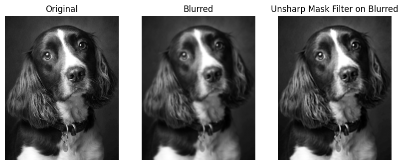
Unsharp masking adds back a scaled high‑frequency residue: Isharp = I + α (I − Gσ*I). I experimented with σ and α on Taj Mahal and another image; DoG‑style sharpening emphasizes edges even more but can introduce halos for large α.
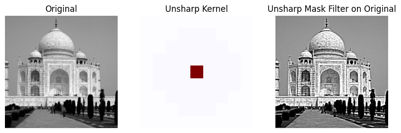
Code — Part 2.1 Unsharp Mask
    gaussian_kernel_1D = getGaussianKernel(9, 3)
    gaussian_kernel_2D = gaussian_kernel_1D @ gaussian_kernel_1D.T
    unit_impulse_kernel = np.zeros_like(gaussian_kernel_2D, dtype=np.float64)
    unit_impulse_kernel[unit_impulse_kernel.shape[0] // 2, unit_impulse_kernel.shape[1] // 2] = 1
    alpha = 2
    unsharp_kernel = (1+alpha)*unit_impulse_kernel - alpha*gaussian_kernel_2D

    img = np.array(Image.open("taj.jpg").convert("L"))
    unsharp_img = convolve2d(img, unsharp_kernel, mode="same", boundary="symm")
    unsharp_img = np.clip(unsharp_img, 0, 255).astype(np.uint8)

    img2 = np.array(Image.open("dog.jpg").convert("L"))
    img2 = downsample(img2, 8)
    gaussian_img2 = convolve2d(img2, gaussian_kernel_2D, mode="same", boundary="symm")
    unsharp_img2 = convolve2d(gaussian_img2, unsharp_kernel, mode="same", boundary="symm")
    unsharp_img2 = np.clip(unsharp_img2, 0, 255).astype(np.uint8)
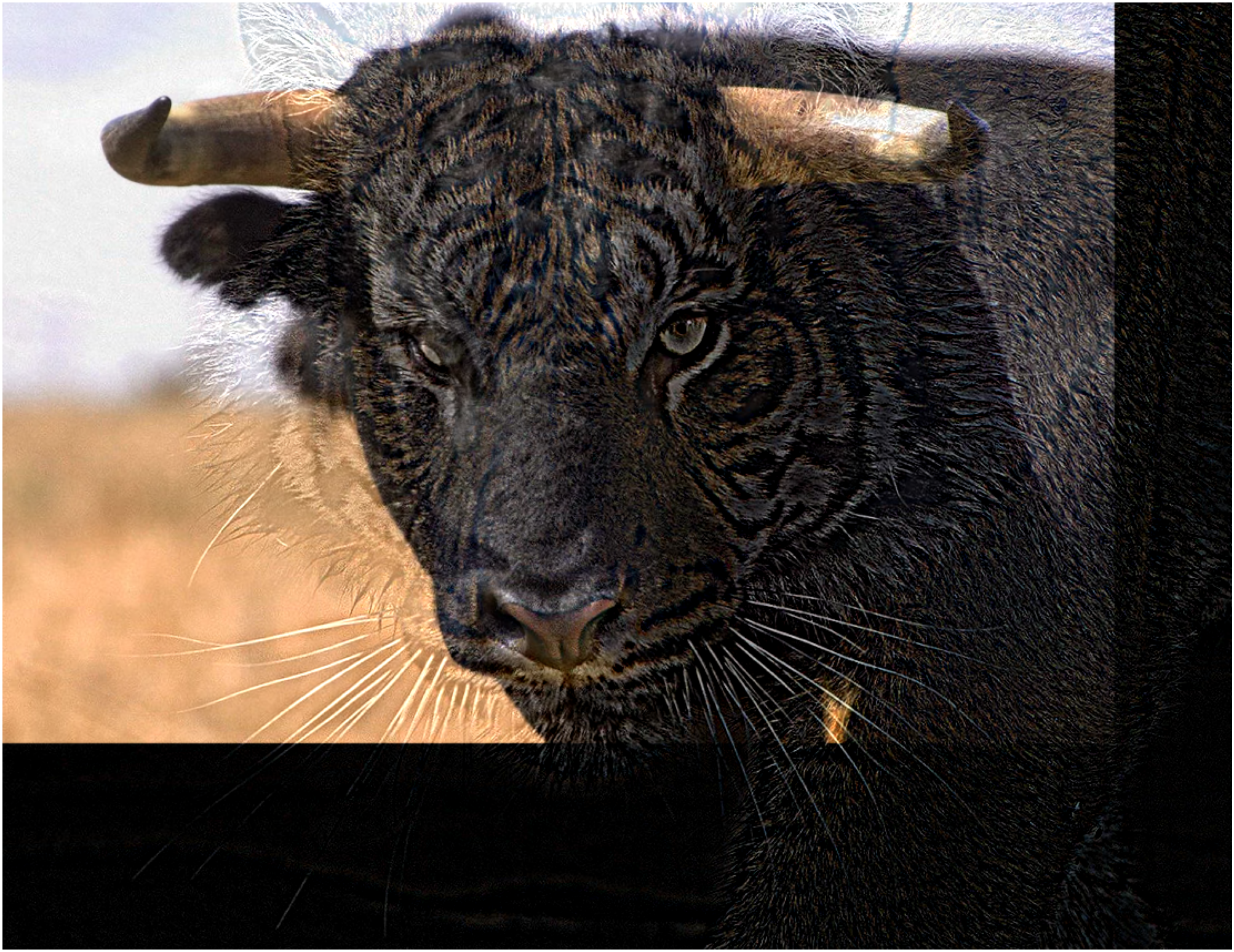
Part 2.2 — Hybrid Images
I align two images with clicked correspondences, low‑pass one and high‑pass the other, then sum. I also visualize the log‑magnitude Fourier spectra of each component and the final hybrid.
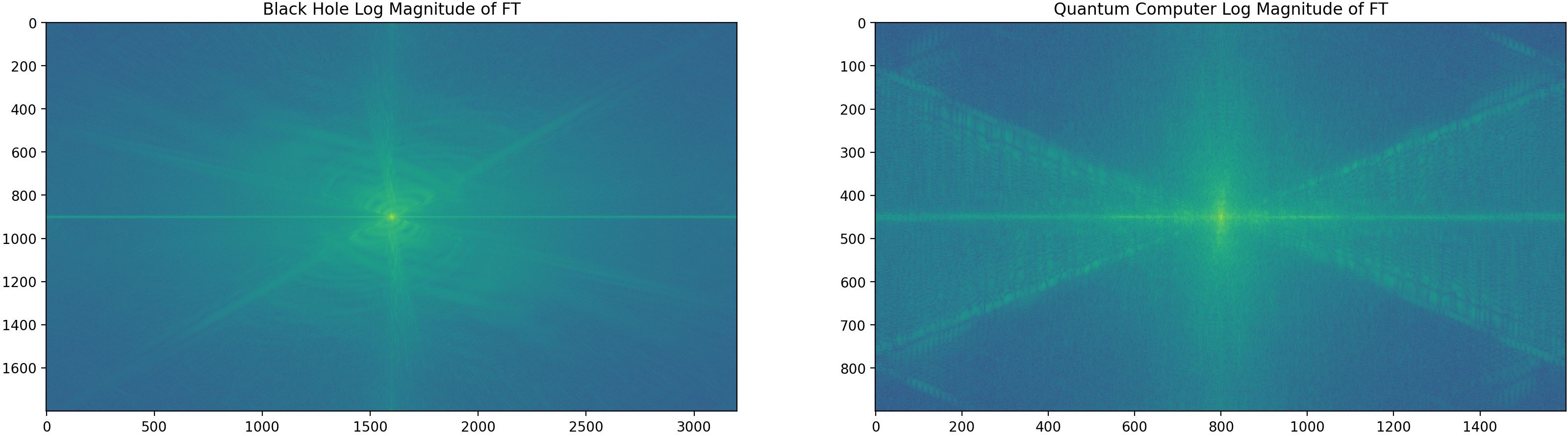
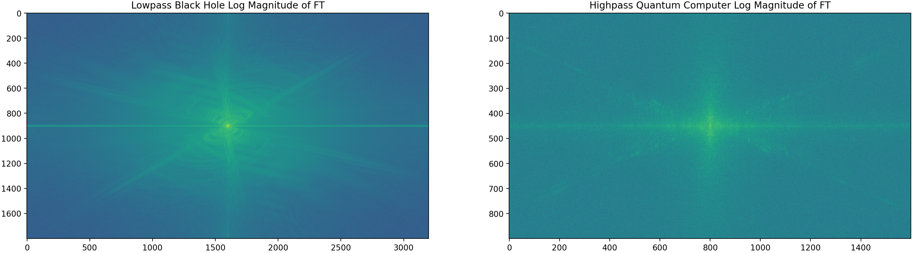
Code — Part 2.2 Hybrid Images
          def hybrid_image(img1, img2, sigma1, sigma2):
            img1_low  = gaussian_filter(img1, sigma=(sigma1, sigma1, 0))
            img2_high = img2 - gaussian_filter(img2, sigma=(sigma2, sigma2, 0))

            return np.clip(img1_low + img2_high, 0.0, 1.0)

          sigma1 = .5
          sigma2 = 5
          hybrid = hybrid_image(im1, im2, sigma1, sigma2)
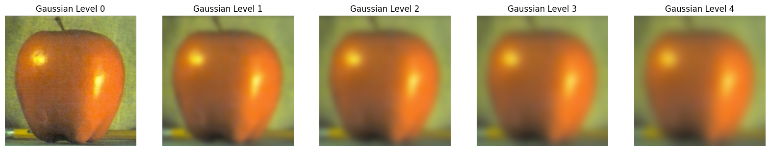
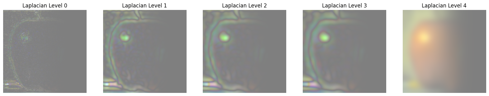
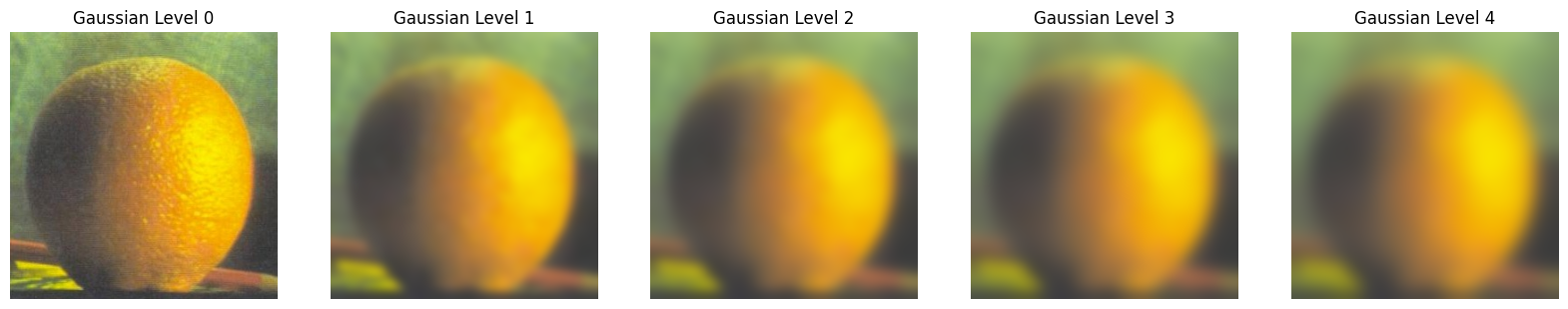
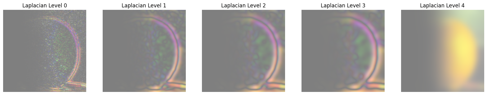
Part 2.3 — Gaussian & Laplacian Stacks
Placeholder: Results and code to be added.
Code — Part 2.3 Gaussian/Laplacian Stack and Horizontal Mask
          def get_gaussian_stack(img, levels=5, sigma=5):
            gaussian_stack = [img]
            for _ in range(1, levels):
                guassian_stack.append(gaussian_filter(guassian_stack[-1], sigma=(sigma, sigma, 0)))
            return guassian_stack

          def get_laplacian_stack(img, levels=5, sigma=5):
              gaussian_stack = get_gaussian_stack(img, levels, sigma)
              laplacian_stack = [gaussian_stack[i] - gaussian_stack[i+1] for i in range(levels-1)] + [gaussian_stack[-1]]
              return gaussian_stack, laplacian_stack

          def get_horizontal_mask(img, direction='right'):
            h, w = img.shape[:2]
            if direction == 'right':
              mask = np.zeros((h, w), np.float32)
              mask[:, :w//2] = 1.0
            else:
              mask = np.ones((h, w), np.float32)
              mask[:, :w//2] = 0
            mask = gaussian_filter(mask, sigma=40)
            return np.dstack([mask, mask, mask])
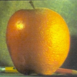
Part 2.4 — Multiresolution Blending
I create Gaussian stacks for a sharp-ramp mask and Laplacian stacks for the two images, then blend per level and collapse. I reproduce the oraple and try two custom blends, including one with an irregular mask.
Code — Part 2.4 Blending and Irregular Mask
    def get_sine_mask(img, cycles=1.0, phase=0.0):
      h, w = img.shape[:2]
      x = np.linspace(0, 2*np.pi*cycles, w, endpoint=False)
      s = np.sin(x + phase)
      line = 0.5 * (1.0 + s)
      mask = np.tile(line[None, :], (h, 1))
      mask = np.clip(mask, 0.0, 1.0)
      mask = gaussian_filter(mask, sigma=20)
      return np.dstack([mask, mask, mask]).astype(np.float32)


    def blend_multires(im1, im2, mask, levels=6, sigma=2):
      guassian_stack1, laplacian_stack1 = get_gaussian_stack(im1, levels, sigma), get_laplacian_stack(im1, levels, sigma)[1]
      guassian_stack2, laplacian_stack2 = get_gaussian_stack(im2, levels, sigma), get_laplacian_stack(im2, levels, sigma)[1]
      guassian_stack_mask = get_gaussian_stack(mask, levels, sigma)

      blends = [guassian_stack_mask[i]*laplacian_stack1[i] + (1.0 - guassian_stack_mask[i])*laplacian_stack2[i] for i in range(levels)]
      out = blends[-1].copy()
      for i in range(levels-2, -1, -1):
          out = out + blends[i]
      return np.clip(out, 0.0, 1.0)

    B = plt.imread('orange.jpeg') / 255.0
    A = plt.imread('apple.jpeg') / 255.0

    h = min(A.shape[0], B.shape[0])
    w = min(A.shape[1], B.shape[1])

    A = A[:h,:w]
    B = B[:h,:w]

    mask = get_horizontal_mask(A)
    out = blend_multires(A, B, mask, 6, 5)
Most Important Takeaway
In both edge detection and blending, frequency‑aware smoothing (Gaussian/DoG and mask pyramids) is the key to suppressing noise and seams while preserving perceptually salient structure.
Deliverables Checklist
- 1.1 Convolution (numpy‑only) + comparison to SciPy; boundary/runtime notes.
- 1.2 Partial derivatives, gradient magnitude, binarized edge image (threshold choice justified).
- 1.3 Gaussian construction, DoG filters visualized, results vs finite differences.
- 2.1 Unsharp mask on Taj + one other; vary amount; show blurred/high‑freq/sharpened.
- 2.2 Three hybrids (Derek+Nutmeg + two originals); one with FT visualizations.
- 2.3/2.4 Gaussian & Laplacian stacks visualized; Oraple reproduction; two custom blends (one irregular mask).
- Clarity: organized webpage with captions and concise explanations.