Projects 3A & 3B — Planar Rectification, Mosaics & Automatic Stitching

Overview

This combined page covers 3A (manual correspondences → homography → inverse warping → mosaics) and 3B (automatic corner detection, patch descriptors, feature matching, RANSAC homography, and mosaics).

What problem are we solving? Given overlapping photos of the same scene, align them onto a shared coordinate system and blend them into a single panorama. 3A solves the geometry with human-picked correspondences; 3B automates the correspondences and makes the pipeline end-to-end.

1. 3A: pick point pairs, solve a homography, inverse-warp images, and feather-blend.
2. 3B: detect corners, extract descriptors, match with a ratio test, run RANSAC, warp & blend.

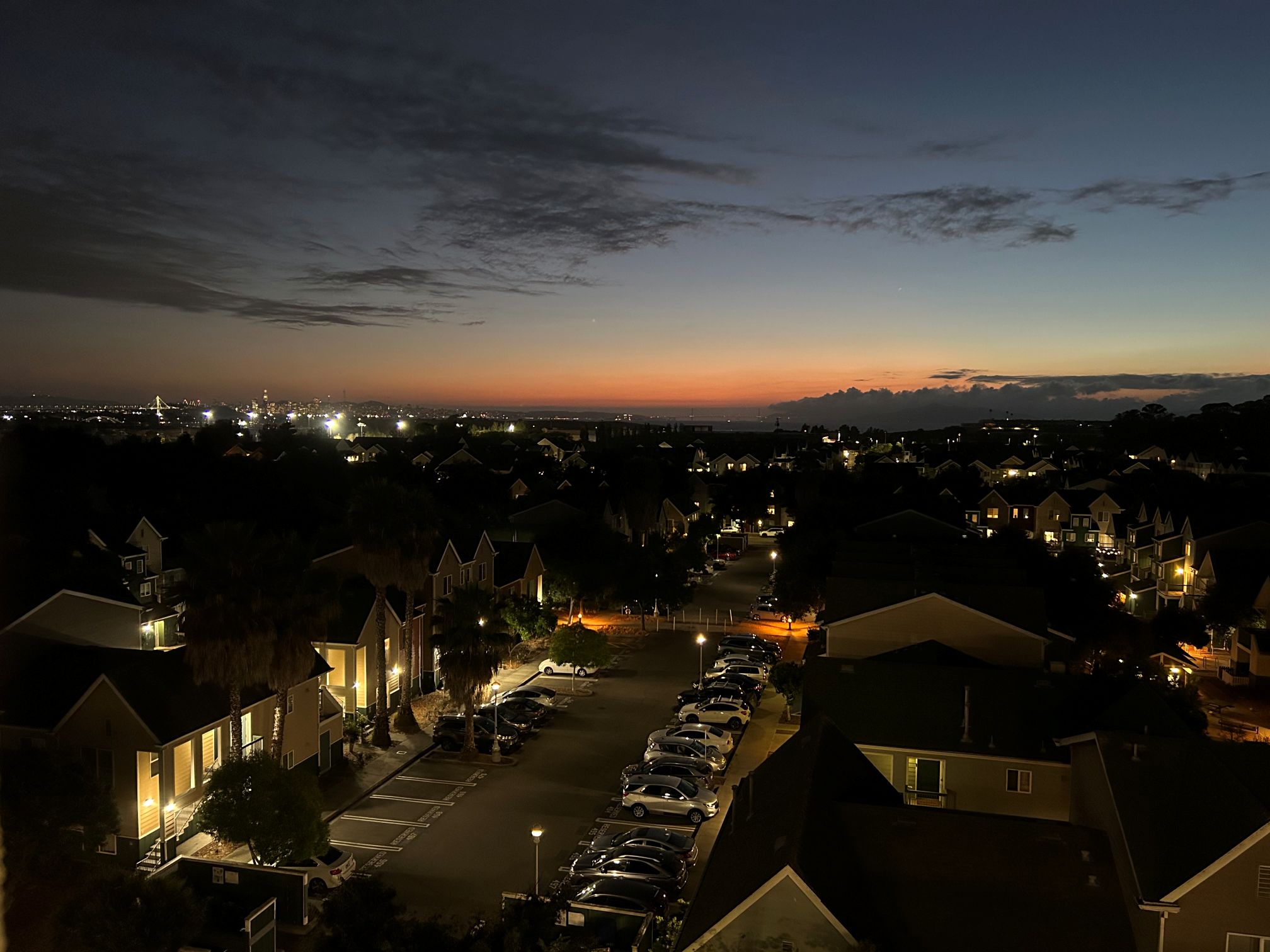
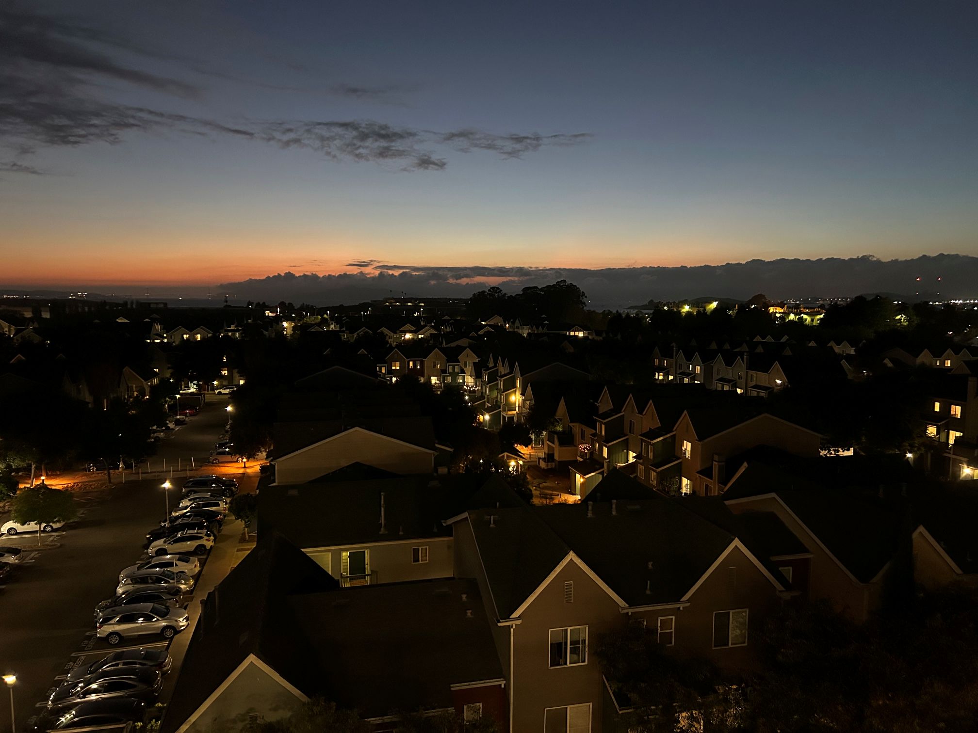
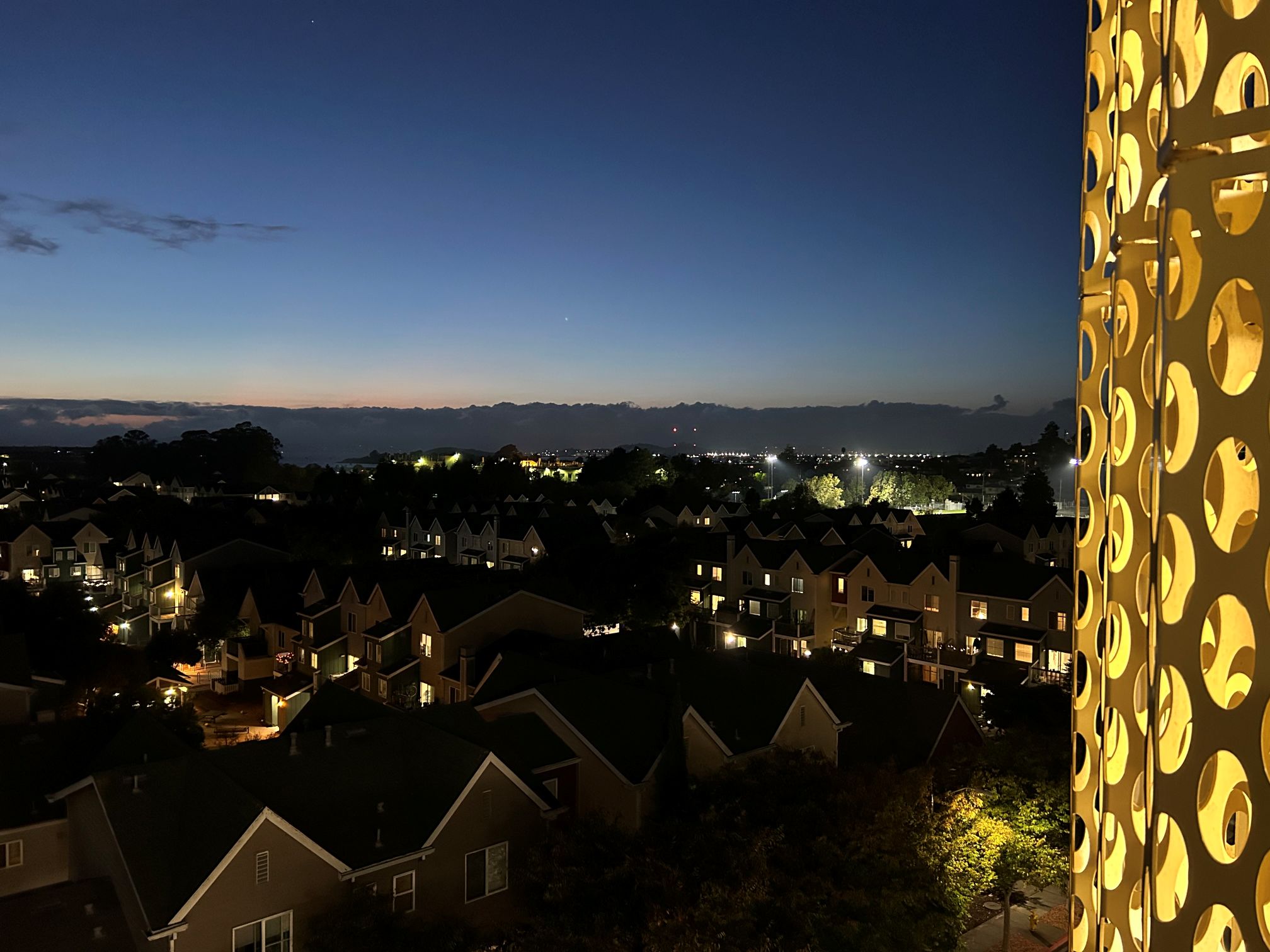
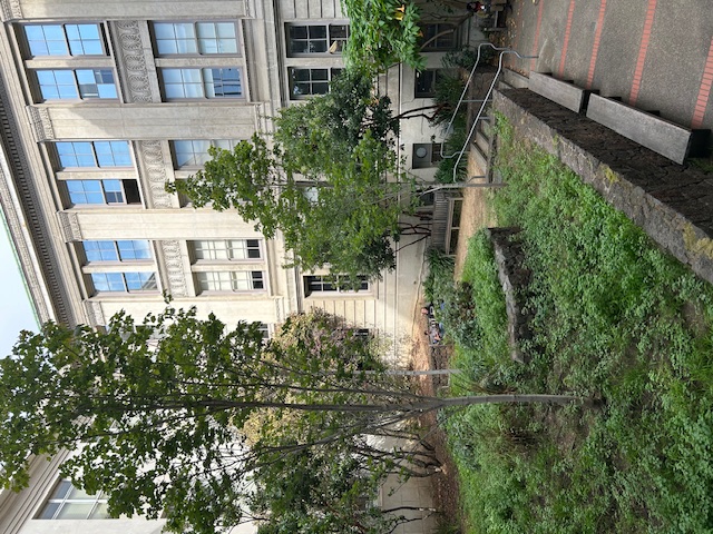
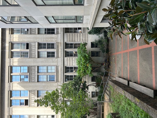
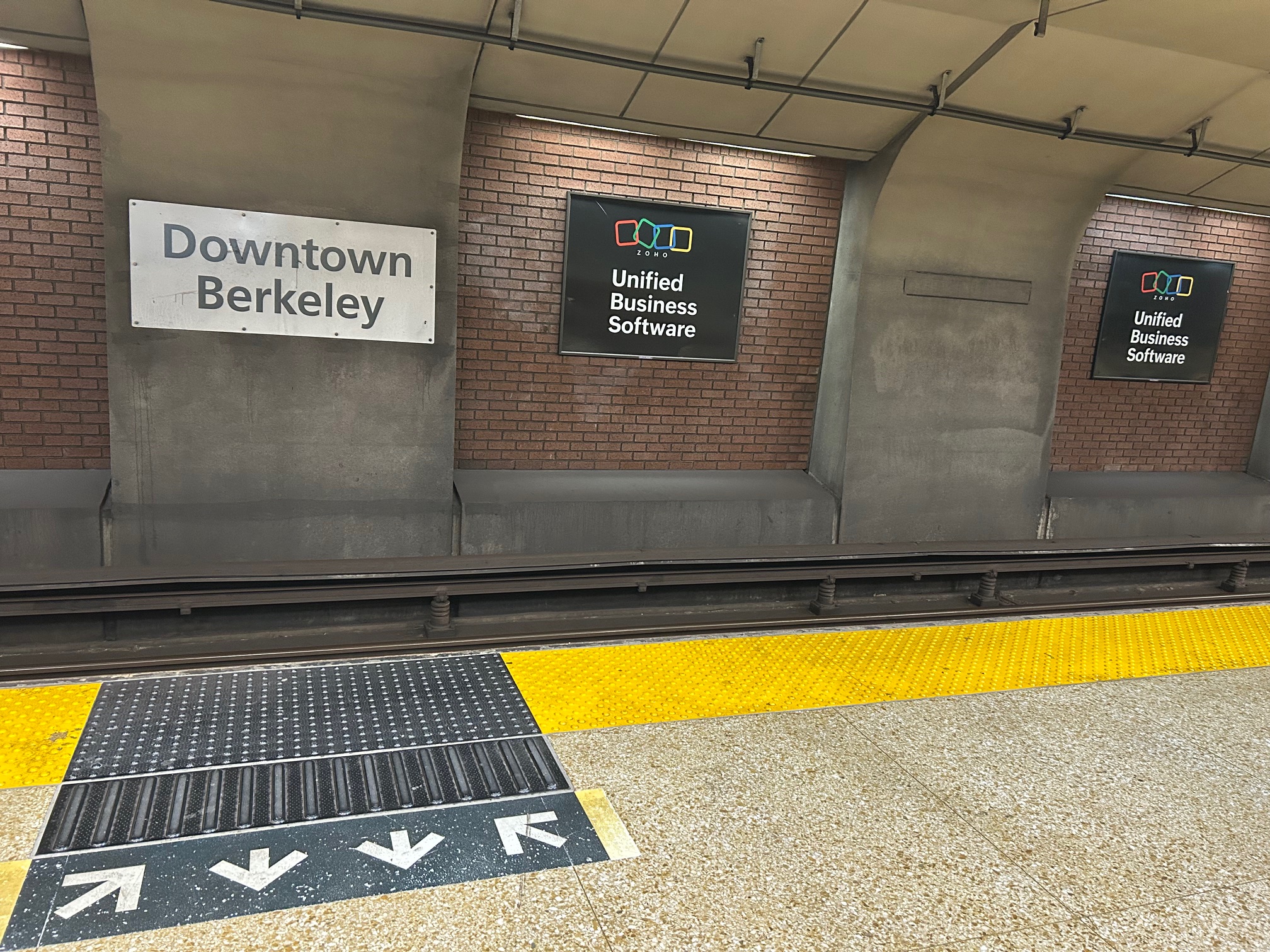
A.1 – Raw Inputs (Project 3A)

The 3A portion uses overlapping photos (three per scene) for mosaics and two oblique shots for rectification examples. Below, we also include the I/O helpers used across 3A so you can see the exact pixel plumbing.

Implementation — EXIF-aware I/O helpers

def read_image(path: str) -> np.ndarray:
    image = Image.open(path)
    image = ImageOps.exif_transpose(image)
    array = np.asarray(image).astype(np.float32) / 255.0
    if array.ndim == 2:
        array = np.stack([array, array, array], axis=-1)
    return array

def save_image(path: str, array: np.ndarray):
    os.makedirs(os.path.dirname(path), exist_ok=True)
    array8 = (np.clip(array, 0, 1) * 255).astype(np.uint8)
    Image.fromarray(array8).save(path, exif=b"")

def to_grayscale(rgb: np.ndarray) -> np.ndarray:
    if rgb.ndim == 2:
        return rgb.astype(np.float32)
    r, g, b = rgb[..., 0], rgb[..., 1], rgb[..., 2]
    return (0.2989 * r + 0.5870 * g + 0.1140 * b).astype(np.float32)

Walkthrough. read_image loads and applies EXIF orientation so pixels match on-screen orientation; returns float32 in [0,1]. If grayscale, it replicates to 3 channels so later code expecting RGB doesn’t break. save_image clips, converts to uint8, and strips EXIF to avoid double rotations. to_grayscale uses standard luminance weights.

Rectification sources

A.2 – Homography (Manual Correspondences → 3×3 H)

A homography is a 3×3 matrix that maps any point on a plane from one image to another. In 3A, we select corresponding points by hand and then solve for H using a numerically stable, normalized DLT.

Implementation — Normalized DLT

def _normalize_points(xy: np.ndarray):
    mu = xy.mean(axis=0)
    d  = np.sqrt(((xy - mu) ** 2).sum(axis=1)).mean()
    s  = np.sqrt(2.0) / max(d, 1e-8)
    T  = np.array([[s, 0, -s * mu[0]],
                   [0, s, -s * mu[1]],
                   [0, 0, 1.0]], dtype=np.float64)
    xy_h = np.c_[xy, np.ones(len(xy))]
    xy_n = (T @ xy_h.T).T
    return T, xy_n[:, :2]

def dlt_homography(xy_src: np.ndarray, xy_dst: np.ndarray) -> np.ndarray:
    assert xy_src.shape == xy_dst.shape and xy_src.shape[0] >= 4
    T_src, src_n = _normalize_points(xy_src)
    T_dst, dst_n = _normalize_points(xy_dst)
    A = []
    for (x, y), (u, v) in zip(src_n, dst_n):
        A.append([-x, -y, -1, 0, 0, 0, u * x, u * y, u])
        A.append([ 0,  0,  0,-x,-y,-1, v * x, v * y, v])
    A = np.asarray(A, dtype=np.float64)
    _, _, Vt = np.linalg.svd(A)
    Hn = Vt[-1].reshape(3, 3)
    H  = np.linalg.inv(T_dst) @ Hn @ T_src
    if abs(H[2,2]) > 1e-12: H /= H[2,2]
    return H

Walkthrough (deep dive)

1. Collect reliable pairs. Pick at least 4 non‑collinear correspondences on the same physical plane (e.g., corners of posters, tile intersections). More points (6–12) help average out click noise; spread them across the plane to avoid degeneracy.
2. Normalize both sets. _normalize_points recenters around the mean and scales so the average radius is √2. This makes the linear system well‑conditioned so SVD finds a stable nullspace vector. Skipping normalization often produces wildly different results depending on the coordinate scale.
3. Build the DLT system. Each pair contributes two equations derived from H [x,y,1]^T ∝ [u,v,1]^T. Stacking all rows yields A h = 0 up to scale. We solve for the last singular vector (the direction of minimal error).
4. Denormalize & scale. Map Hn back to pixel space by T_dst^{-1} · Hn · T_src; divide so H[2,2]=1 for readability. This doesn’t change the mapping, just the representation.
5. Sanity checks. (a) Reproject the input points and report the RMS pixel error; you should see sub‑pixel to a few pixels depending on click noise. (b) Visualize epipolar‑looking distortions—if straight lines bend, you probably mixed planes or mis‑clicked.
6. Edge cases. Four nearly collinear points make A rank‑deficient → unstable H. Avoid all points being from a tiny patch: lever arm is too short and errors explode away from the patch.

Applying H to points (numerical safety)

def apply_homography_points(xy: np.ndarray, H: np.ndarray) -> np.ndarray:
    xy_h = np.c_[xy, np.ones(len(xy))]
    uvw  = (H @ xy_h.T).T
    w = uvw[:, 2:3]
    out = np.full((len(xy), 2), np.nan, dtype=np.float64)
    good = np.abs(w) > 1e-8
    if np.any(good):
        out[good[:, 0]] = uvw[good[:, 0], :2] / w[good[:, 0]]
    return out

Why check w? Points that map near the projective horizon (w ≈ 0) would blow up under division. Marking them as NaN prevents downstream crashes and makes debugging footprints easier.

A.3 – Warping & Rectification

Given H from the oblique view to a fronto‑parallel target, we render a rectified image using inverse warping: for each output pixel, we ask “where in the source would this have come from?” and sample there. Inverse warping avoids holes and duplicated pixels.

Implementation — Inverse Warping + Bilinear Sampling

def bilinear_sample(img: np.ndarray, x: float, y: float):
    H, W = img.shape[:2]
    if x < 0 or y < 0 or x > W - 1 or y > H - 1:
        return None, False
    x0 = int(np.floor(x)); x1 = min(x0 + 1, W - 1)
    y0 = int(np.floor(y)); y1 = min(y0 + 1, H - 1)
    ax = x - x0; ay = y - y0
    I00 = img[y0, x0]; I10 = img[y0, x1]
    I01 = img[y1, x0]; I11 = img[y1, x1]
    I0 = (1 - ax) * I00 + ax * I10
    I1 = (1 - ay) * I01 + ay * I11
    return (1 - ay) * I0 + ay * I1, True

def inverse_warp_to_canvas(src_img: np.ndarray, H_inv: np.ndarray,
                           out_h: int, out_w: int, offset_xy: tuple[int,int],
                           mode: str = "bilinear"):
    ox, oy = offset_xy
    C = src_img.shape[2] if src_img.ndim == 3 else 1
    out   = np.zeros((out_h, out_w, C), dtype=np.float32)
    alpha = np.zeros((out_h, out_w), dtype=np.float32)
    sampler = bilinear_sample if mode == "bilinear" else sample_nearest
    h0, h1, h2 = H_inv[0], H_inv[1], H_inv[2]
    for Y in range(out_h):
        for X in range(out_w):
            Xc, Yc = float(X), float(Y)
            w = h2[0]*(Xc-ox) + h2[1]*(Yc-oy) + h2[2]
            if abs(w) < 1e-12: continue
            x = (h0[0]*(Xc-ox) + h0[1]*(Yc-oy) + h0[2]) / w
            y = (h1[0]*(Xc-ox) + h1[1]*(Yc-oy) + h1[2]) / w
            val, ok = sampler(src_img, x, y)
            if ok:
                out[Y, X] = val
                alpha[Y, X] = 1.0
    return out, alpha

Walkthrough (pixel‑accurate rectification)

1. Target geometry. Decide the rectified canvas size by measuring the expected real‑world aspect ratio (e.g., poster width:height) or by warping four corners and taking their bounding box. Bigger canvases preserve detail but cost time.
2. Back‑project each output pixel. We pre‑split H⁻¹ rows (h0,h1,h2) so the tight inner loop only does a handful of multiplies and one division.
3. Interpolate. Bilinear combines the four nearest neighbors weighted by fractional offsets; it smooths jaggies compared to nearest but preserves edges fairly well.
4. Validity mask. We write 1 into alpha only when (x,y) lies inside the source bounds. This mask becomes crucial when blending multiple views.
5. Offsets. offset_xy lets us place warped content with negative coordinates onto a positive‑indexed array. For single‑view rectification it’s usually (0,0); for mosaics it’s often nonzero.
6. Quality tips. (a) If aliasing appears on fine patterns, pre‑blur slightly before warping. (b) If borders look dark, ensure out‑of‑bounds samples return ok=False rather than zeros that get averaged in.

Takeaway. Nearest is fast but jaggy; bilinear trades a tiny bit of sharpness for much smoother edges. For mosaics you can consider bicubic or Lanczos, but bilinear is typically sufficient.

A.4 – Panoramic Mosaics (Project 3A)

We register all images to a single reference, estimate a canvas that fits every warped footprint, render each image with inverse warping, and feather‑blend overlaps so seams fade away.

Implementation — Canvas sizing & Feathered blending

def image_corners_wh(width: int, height: int) -> np.ndarray:
    return np.array([[0, 0], [width - 1, 0], [width - 1, height - 1], [0, height - 1]], dtype=np.float64)

def warp_footprint_bbox(width: int, height: int, H_map: np.ndarray):
    corners = image_corners_wh(width, height)
    warped  = apply_homography_points(corners, H_map)
    xs, ys  = warped[:, 0], warped[:, 1]
    if np.all(np.isnan(xs)) or np.all(np.isnan(ys)):
        return 0.0, 0.0, 0.0, 0.0
    return np.nanmin(xs), np.nanmax(xs), np.nanmin(ys), np.nanmax(ys)

def global_canvas_from_maps(image_shapes: List[Tuple[int, int]], H_maps: List[np.ndarray]):
    xs_min, xs_max, ys_min, ys_max = [], [], [], []
    for (H, W), Hc in zip(image_shapes, H_maps):
        xmin, xmax, ymin, ymax = warp_footprint_bbox(W, H, Hc)
        xs_min.append(xmin); xs_max.append(xmax)
        ys_min.append(ymin); ys_max.append(ymax)
    Xmin, Xmax = np.floor(min(xs_min)), np.ceil(max(xs_max))
    Ymin, Ymax = np.floor(min(ys_min)), np.ceil(max(ys_max))
    canvas_w = int(max(1, Xmax - Xmin))
    canvas_h = int(max(1, Ymax - Ymin))
    offset   = (-int(Xmin), -int(Ymin))
    return canvas_h, canvas_w, offset

def center_falloff_weights(alpha: np.ndarray) -> np.ndarray:
    H, W = alpha.shape
    y = np.arange(H)[:, None]
    x = np.arange(W)[None, :]
    d_left, d_right = x, (W - 1 - x)
    d_top,  d_bot   = y, (H - 1 - y)
    d = np.minimum(np.minimum(d_left, d_right), np.minimum(d_top, d_bot))
    d = d * alpha
    m = d.max() if d.max() > 0 else 1.0
    return d / m

def feather_blend(images: List[np.ndarray], alphas: List[np.ndarray]) -> np.ndarray:
    H, W, C = images[0].shape
    accum = np.zeros((H, W, C), dtype=np.float32)
    wsum  = np.zeros((H, W, 1), dtype=np.float32)
    for img, a in zip(images, alphas):
        w = center_falloff_weights(a) * (a > 0).astype(np.float32)
        w = w[..., None]
        accum += w * img
        wsum  += w
    wsum[wsum == 0] = 1.0
    return accum / wsum

Walkthrough (full pipeline)

1. Choose a reference. Pick the most central or sharpest frame as the origin (identity homography). Estimate H for every other image that maps it into this reference frame (manual correspondences in 3A).
2. Predict footprints. Warp each image’s four corners using its H. Taking global min/max over x and y gives the canvas bounds; the negative mins become the offset.
3. Render with masks. For each image, call inverse_warp_to_canvas to get an RGB array and an alpha mask indicating valid pixels. Store both.
4. Feather weights. Convert alpha to a smooth weight that decays near borders so overlaps blend gently instead of creating hard seams. (For even better results, multi‑band blending is a drop‑in upgrade.)
5. Accumulate & normalize. Sum w * I across all images and divide by the sum of weights per pixel. Pixels that only one image covers get weight 1; overlaps become a weighted average.
6. Practical tips. (a) Render the reference frame last or give it slightly higher weights to anchor exposure. (b) If exposures differ a lot, do a quick per‑image gain match in the overlap region before blending.

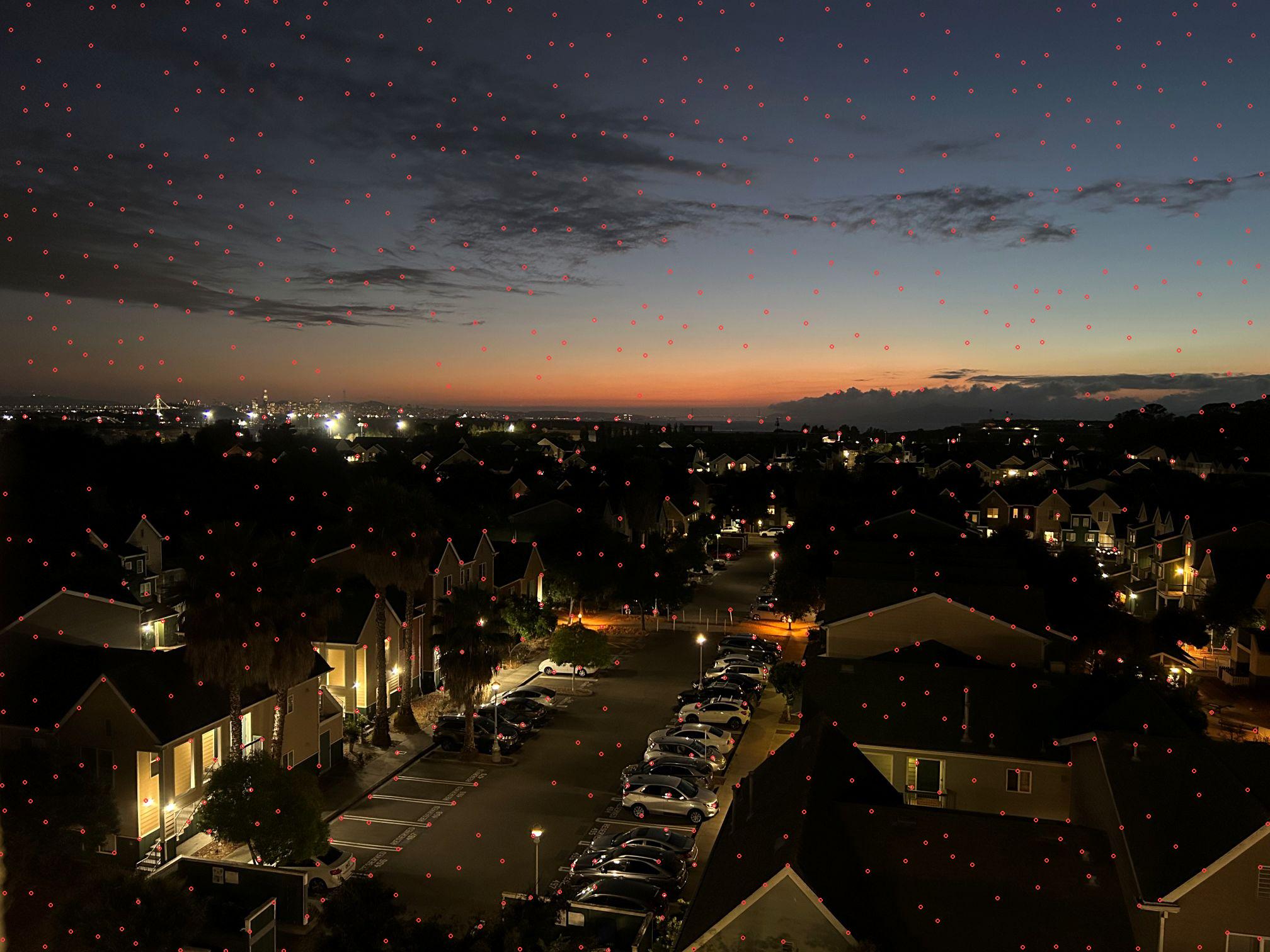
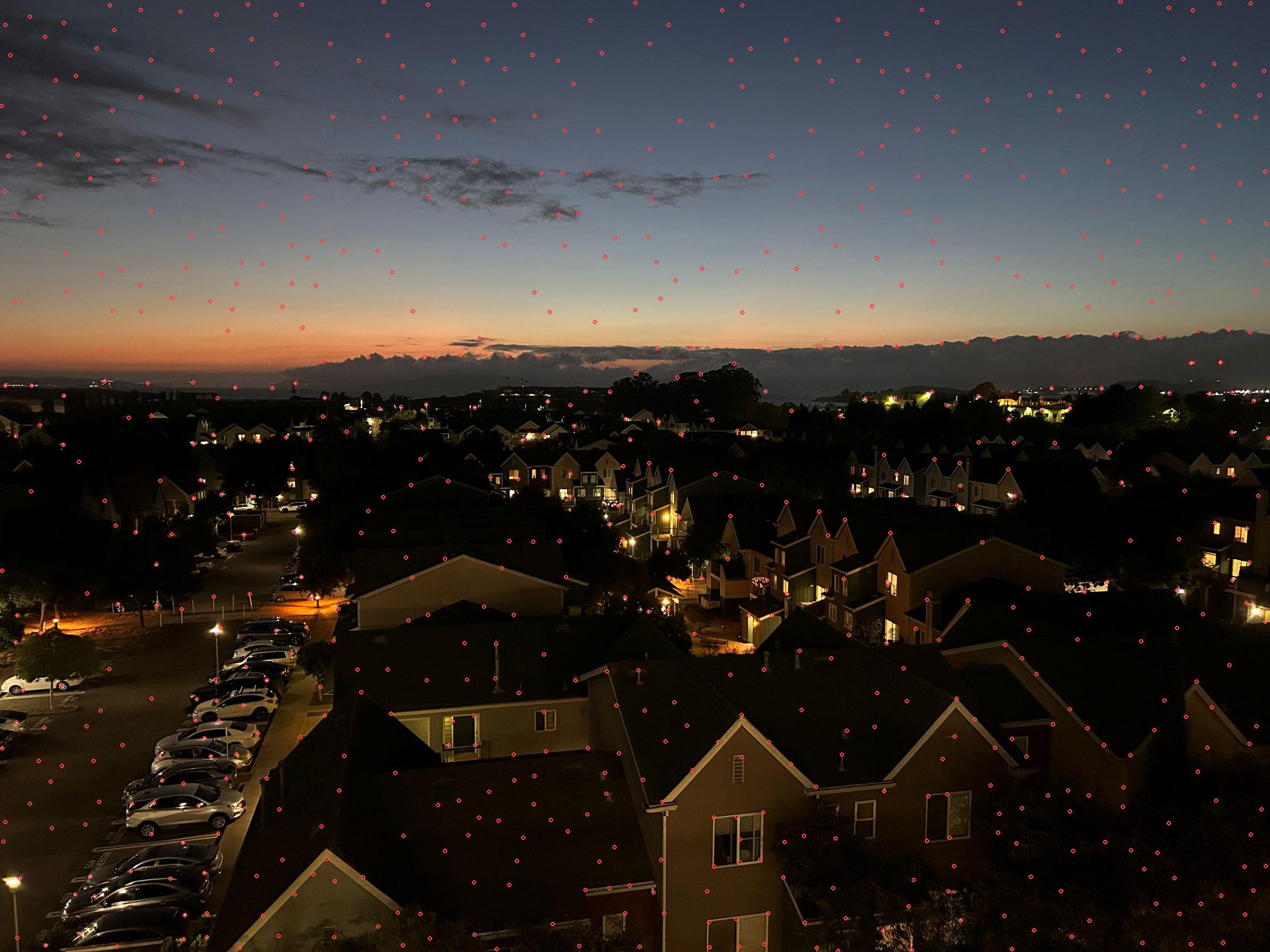
B.1 – Harris Corner Detection

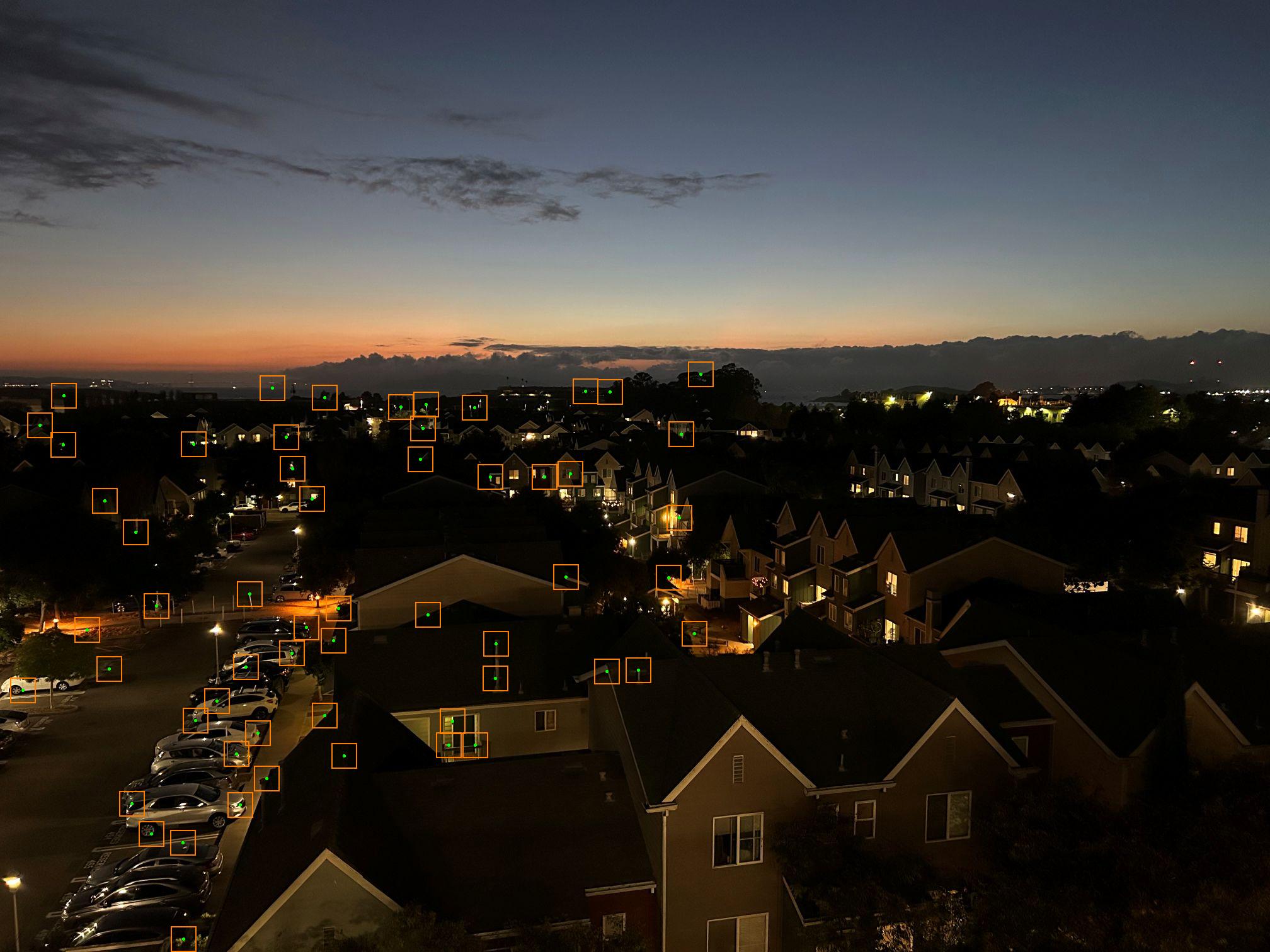
We detect corners with a Harris interest point operator and optionally refine the set with Adaptive Non-Maximal Suppression (ANMS).

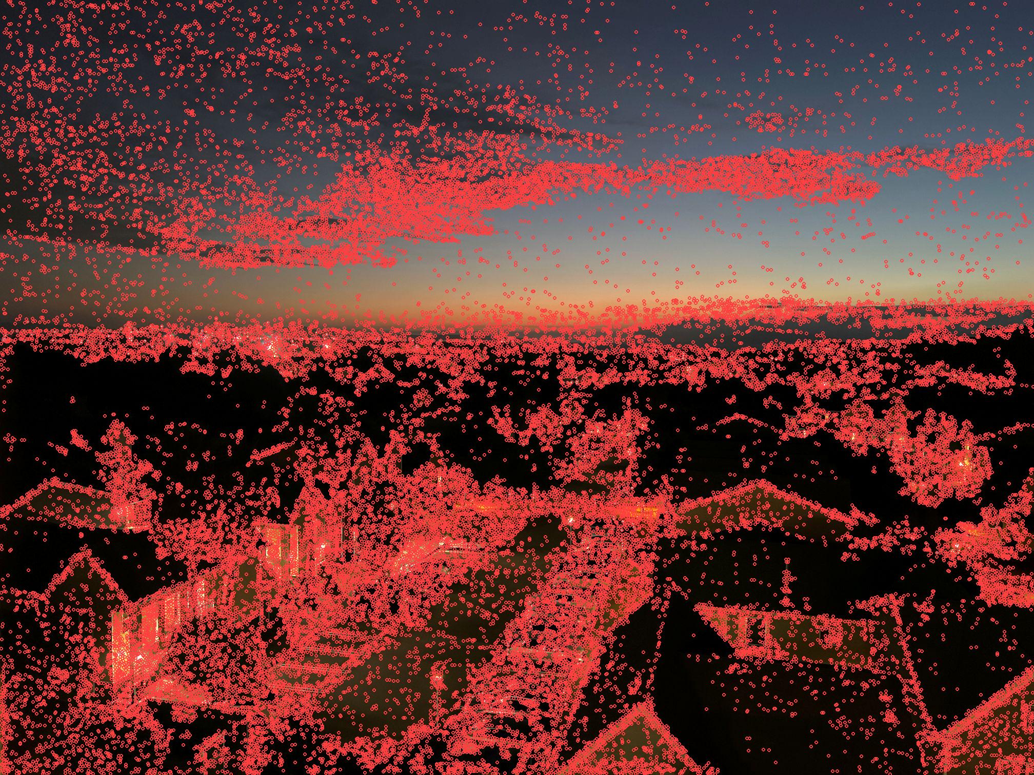
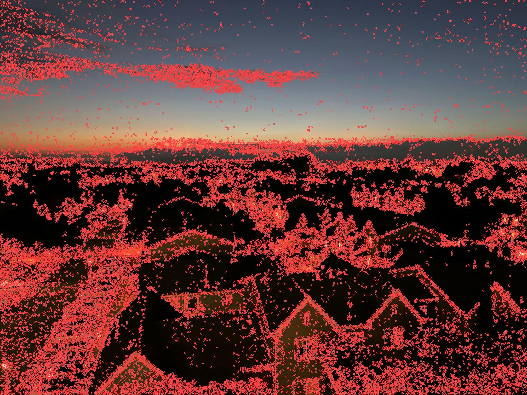
Intuition. A corner is a spot where intensity changes strongly in both directions (think: a checkerboard corner vs. a flat wall). Harris measures how much the image varies around each pixel. High scores indicate good, repeatable points that are easy to re‑find in another photo of the same scene.

Why ANMS? Raw detection can cluster many points in one small area and ignore others. ANMS keeps the strongest points while spreading them out spatially, which improves coverage and makes the later matching step more stable.

Implementation (Harris + ANMS)

def harris_corner_response(gray: np.ndarray, k_coeff: float = harris_k_coeff, window_size: int = harris_window_size) -> np.ndarray:
    sobel_x = np.array([[1, 0, -1], [2, 0, -2], [1, 0, -1]], dtype=np.float32)
    sobel_y = np.array([[1, 2, 1], [0, 0, 0], [-1, -2, -1]], dtype=np.float32)
    grad_x = conv2d_same(gray, sobel_x)
    grad_y = conv2d_same(gray, sobel_y)
    grad_xx, grad_yy, grad_xy = grad_x * grad_x, grad_y * grad_y, grad_x * grad_y
    gauss = gaussian_kernel_2d(window_size if window_size % 2 else window_size + 1, sigma=1.0)
    sum_xx = conv2d_same(grad_xx, gauss)
    sum_yy = conv2d_same(grad_yy, gauss)
    sum_xy = conv2d_same(grad_xy, gauss)
    determinant = sum_xx * sum_yy - sum_xy * sum_xy
    trace = sum_xx + sum_yy
    response = determinant - k_coeff * (trace ** 2)
    r_min, r_max = float(response.min()), float(response.max())
    if r_max > r_min:
        return (response - r_min) / (r_max - r_min)
    return np.zeros_like(response)

def nms_local_maxima(harris_norm: np.ndarray, threshold_relative: float = harris_threshold_relative):
    height, width = harris_norm.shape
    threshold_value = threshold_relative * float(harris_norm.max())
    keep_mask = np.zeros_like(harris_norm, dtype=bool)
    for y in range(1, height - 1):
        for x in range(1, width - 1):
            value = harris_norm[y, x]
            if value < threshold_value:
                continue
            window = harris_norm[y - 1:y + 2, x - 1:x + 2]
            if value == window.max() and np.count_nonzero(window == value) == 1:
                keep_mask[y, x] = True
    ys, xs = np.where(keep_mask)
    vals = harris_norm[ys, xs]
    return xs.astype(np.float32), ys.astype(np.float32), vals.astype(np.float32)

def adaptive_nms(x_coords: np.ndarray, y_coords: np.ndarray, strengths: np.ndarray, top_k: int = max_keypoints_after_anms):
    count = len(x_coords)
    if count == 0:
        return x_coords, y_coords, strengths
    order = np.argsort(-strengths)
    x_coords, y_coords, strengths = x_coords[order], y_coords[order], strengths[order]
    radii_sq = np.full(count, np.inf, dtype=np.float32)
    for i in range(1, count):
        dx = x_coords[:i] - x_coords[i]
        dy = y_coords[:i] - y_coords[i]
        dist2 = dx * dx + dy * dy
        radii_sq[i] = float(np.min(dist2)) if i > 0 else np.inf
    radii_sq[0] = np.inf
    selected = np.argsort(-radii_sq)[:min(top_k, count)]
    return x_coords[selected], y_coords[selected], strengths[selected]

Walkthrough. harris_corner_response builds x/y gradients with Sobel filters, aggregates squared terms with a Gaussian window (approximating the structure tensor), and returns a normalized Harris score per pixel. nms_local_maxima keeps only strict 3×3 peaks above a relative threshold. adaptive_nms then sorts by strength and assigns each point a suppression radius to the nearest stronger point; we keep the largest radii so corners are spatially spread out and stable for matching.

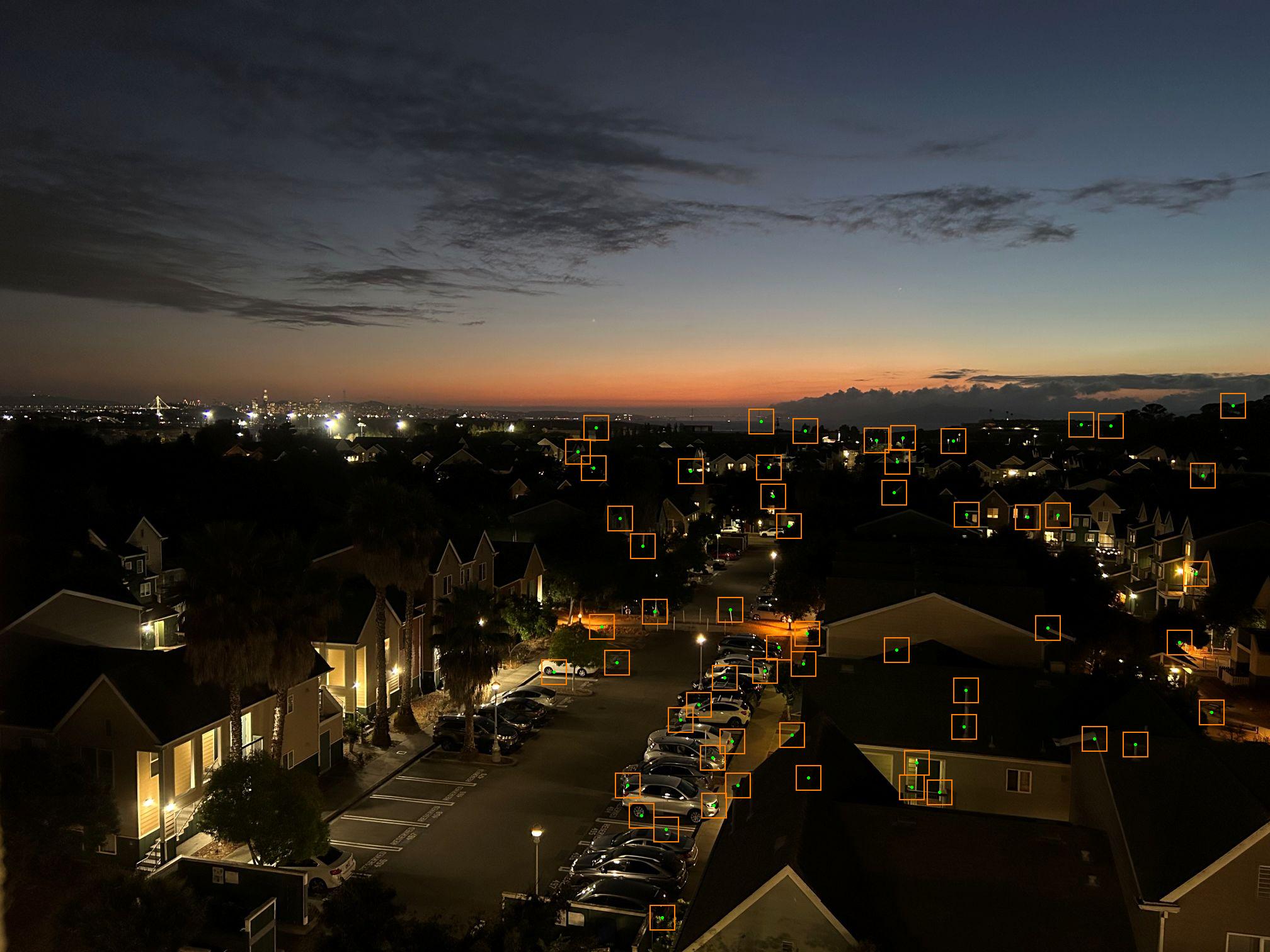
B.2 – Feature Descriptor Extraction

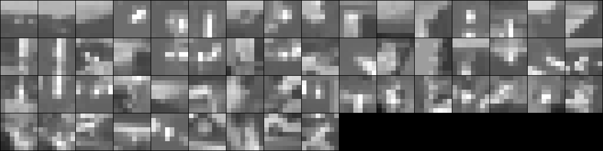
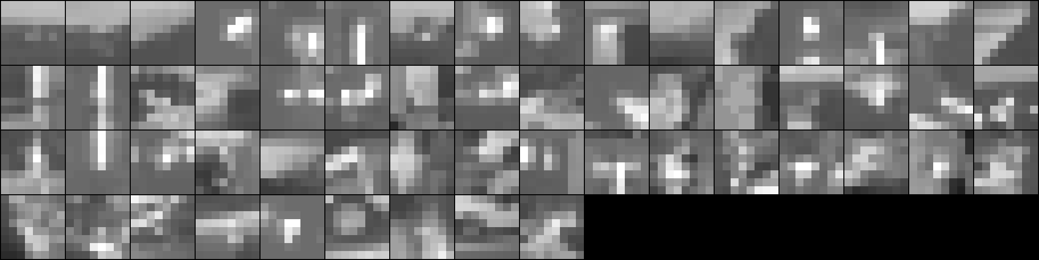
Around each selected corner, we sample a 40×40 window (blurred / downsampled) to produce a normalized 8×8 grayscale descriptor (bias–gain normalized). Below are some of the Set 1 overlays (40×40 boxes with center points at some corners) and the corresponding 8×8 descriptor montages.

Implementation (Patch → 8×8 → z‑score)

def extract_square_patch(gray: np.ndarray, center_x: float, center_y: float, size: int = 40) -> np.ndarray:
    height, width = gray.shape
    half = size // 2
    x0, y0 = int(round(center_x)) - half, int(round(center_y)) - half
    x1, y1 = x0 + size, y0 + size
    if x0 < 0 or y0 < 0 or x1 > width or y1 > height:
        return None
    return gray[y0:y1, x0:x1].copy()

def resize_patch_to_8x8(patch_40: np.ndarray) -> np.ndarray:
    patch_uint8 = (np.clip(patch_40, 0, 1) * 255).astype(np.uint8)
    image = Image.fromarray(patch_uint8)
    image8 = image.resize((8, 8), resample=Image.BILINEAR)
    return np.asarray(image8).astype(np.float32) / 255.0

def normalize_descriptor_vector(patch_8x8: np.ndarray) -> np.ndarray:
    vector = patch_8x8.flatten().astype(np.float32)
    mean_value = float(np.mean(vector))
    std_value = float(np.std(vector))
    if std_value < 1e-6:
        std_value = 1.0
    return (vector - mean_value) / std_value

def build_patch_descriptors(gray: np.ndarray, x_coords: np.ndarray, y_coords: np.ndarray):
    descriptor_list, kept_x, kept_y, display_patches = [], [], [], []
    for x_val, y_val in zip(x_coords, y_coords):
        patch = extract_square_patch(gray, x_val, y_val, size=40)
        if patch is None:
            continue
        patch8 = resize_patch_to_8x8(patch)
        descriptor = normalize_descriptor_vector(patch8)
        descriptor_list.append(descriptor)
        kept_x.append(x_val)
        kept_y.append(y_val)
        display_patches.append(normalize_patch_for_display(patch8))
    if len(descriptor_list) == 0:
        return np.zeros((0, 64), dtype=np.float32), np.array([]), np.array([]), np.zeros((0, 8, 8), dtype=np.float32)
    return np.vstack(descriptor_list), np.array(kept_x), np.array(kept_y), np.stack(display_patches, axis=0)

Walkthrough. We crop a 40×40 window centered on each corner (skip if it would go out of bounds), bilinearly resize to 8×8 to reduce noise and standardize size, then flatten and z‑score the 64 pixels to remove brightness/contrast bias. The helper returns both the numeric descriptors (for matching) and display‑normalized patches (for the montages you see above).

Each corner produces a 40×40 patch (bounds-checked), which is bilinearly resized to 8×8 and z-score normalized to suppress illumination bias and gain differences.

Step‑by‑step (from scratch):

1. For each selected corner, crop a 40×40 grayscale window centered on it.
2. Downsample that window to 8×8 using bilinear interpolation. This reduces noise and makes all descriptors the same size.
3. Normalize the 64 values: subtract the mean and divide by the standard deviation (z‑score). This makes descriptors less sensitive to brightness/exposure.
4. Optionally visualize: draw 40×40 boxes on the original images and show grids of the 8×8 patches (shown above for Set 1).

B.3 – Feature Matching

We compute nearest neighbors in descriptor space and apply Lowe’s ratio test to keep reliable correspondences.

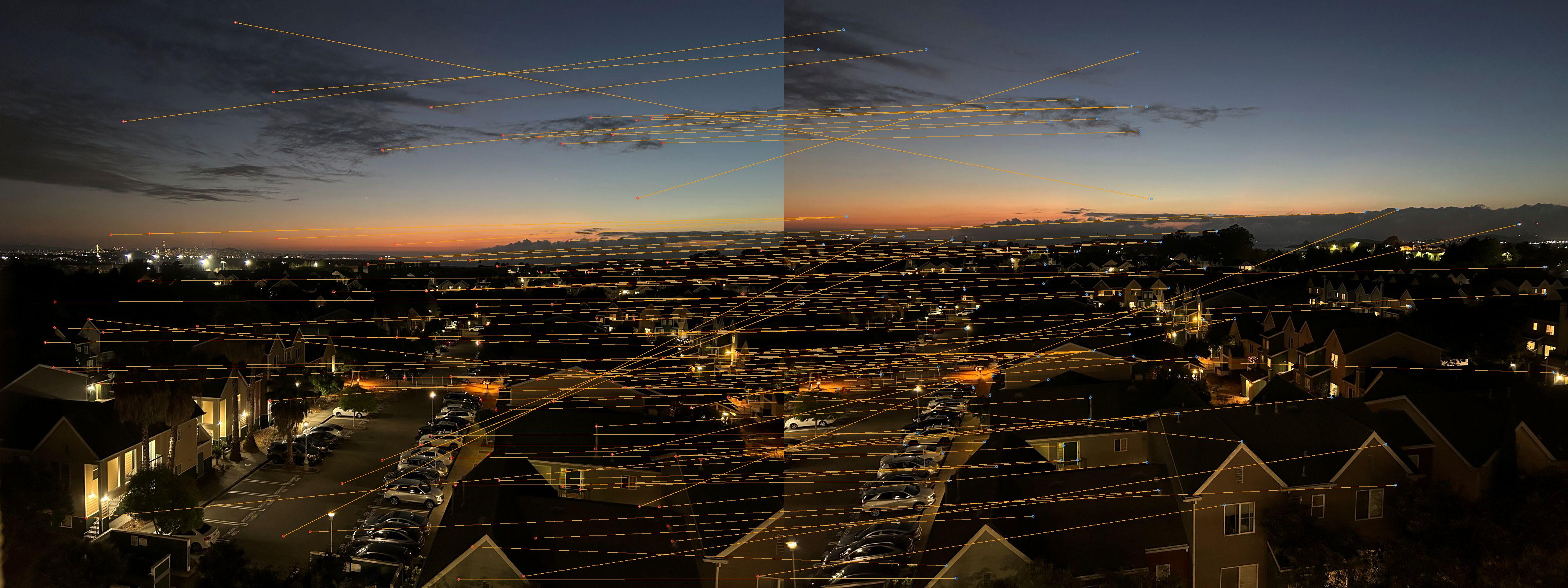
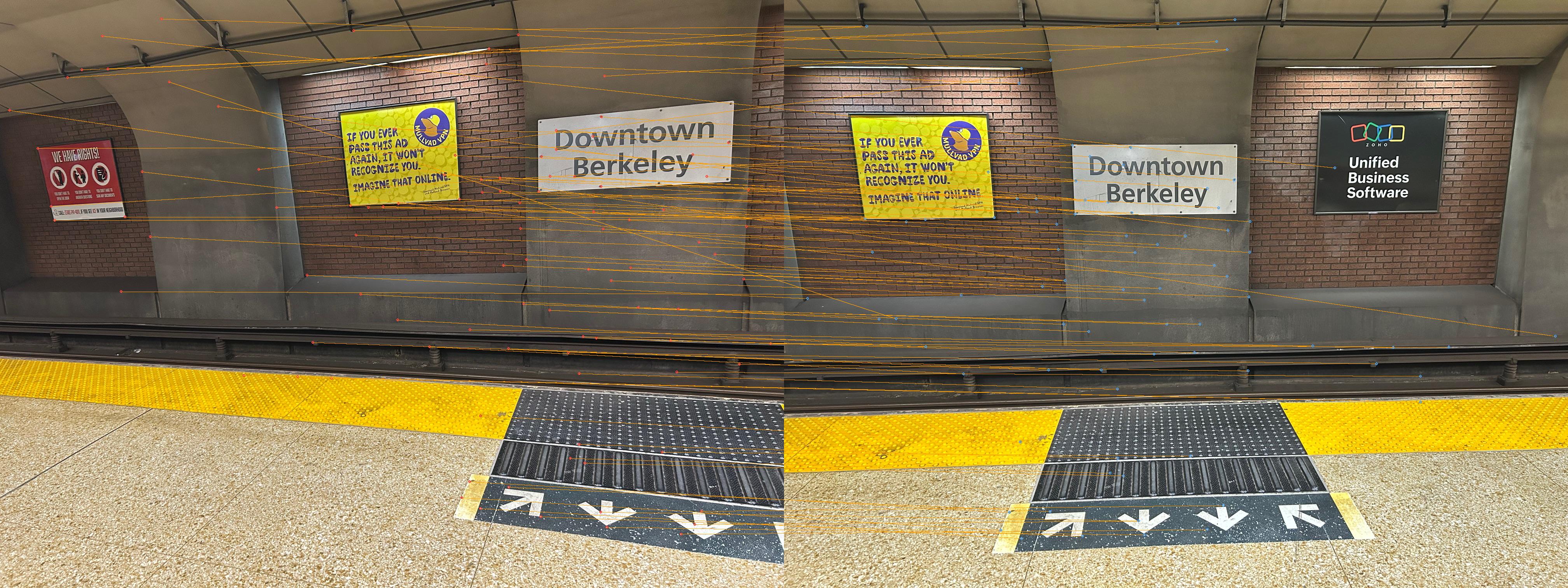
What is a “match”? After we convert patches to 64‑D vectors, we can measure how similar two patches are by their Euclidean distance (small = similar). For each left‑image descriptor we find its nearest neighbor in the right image.

Why the ratio test? Sometimes the best and second‑best matches are similarly good—an ambiguity that often means the match isn’t reliable. The ratio test accepts a pair only if “best” is noticeably better than “runner‑up”. This prunes many false pairs while keeping the real ones.

Implementation (Lowe ratio matching)

def match_with_lowe_ratio(descriptors_left: np.ndarray, descriptors_right: np.ndarray, ratio_threshold: float = lowe_ratio_threshold):
    matches = []
    if len(descriptors_left) == 0 or len(descriptors_right) == 0:
        return matches
    distances = np.sum((descriptors_left[:, None, :] - descriptors_right[None, :, :]) ** 2, axis=2)
    for idx_left in range(descriptors_left.shape[0]):
        row = distances[idx_left]
        order = np.argsort(row)
        idx_right_best = int(order[0])
        idx_right_next = int(order[1]) if len(order) > 1 else int(order[0])
        best_dist = float(row[idx_right_best])
        next_dist = float(row[idx_right_next])
        if next_dist == 0:
            continue
        if best_dist / next_dist < ratio_threshold:
            matches.append((idx_left, idx_right_best, best_dist, next_dist))
    return matches

Walkthrough. We compute the dense left‑to‑right distance matrix once, then for each left descriptor pick the smallest (best) and second‑smallest (runner‑up) distances. A match is kept only if best/next < ratio_threshold (default 0.7), which filters out ambiguous pairs that are likely false.

For each left descriptor, we take the best and second-best right matches by L2 distance and accept the match if the best/second-best ratio is below 0.7.

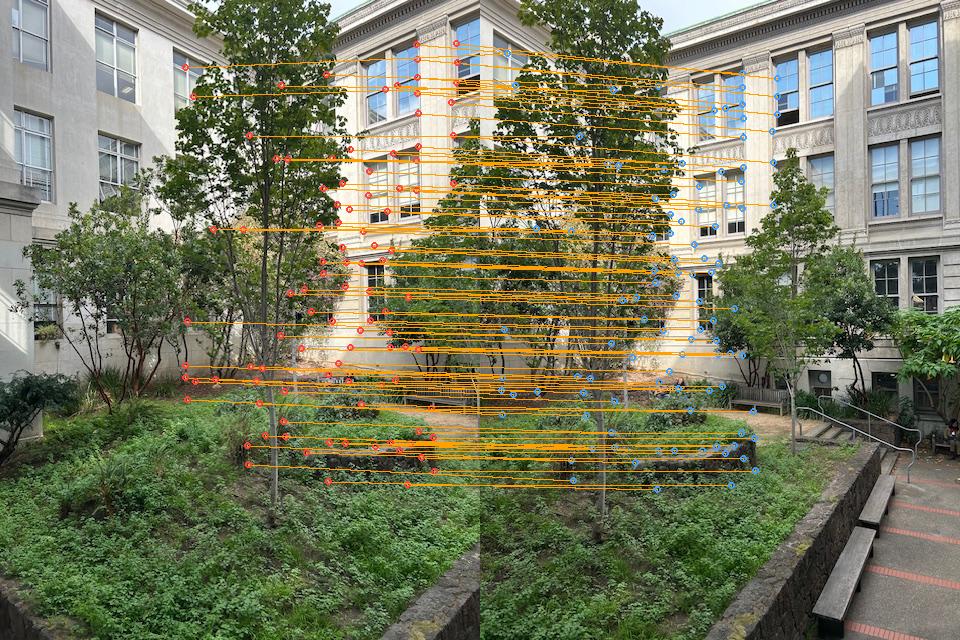
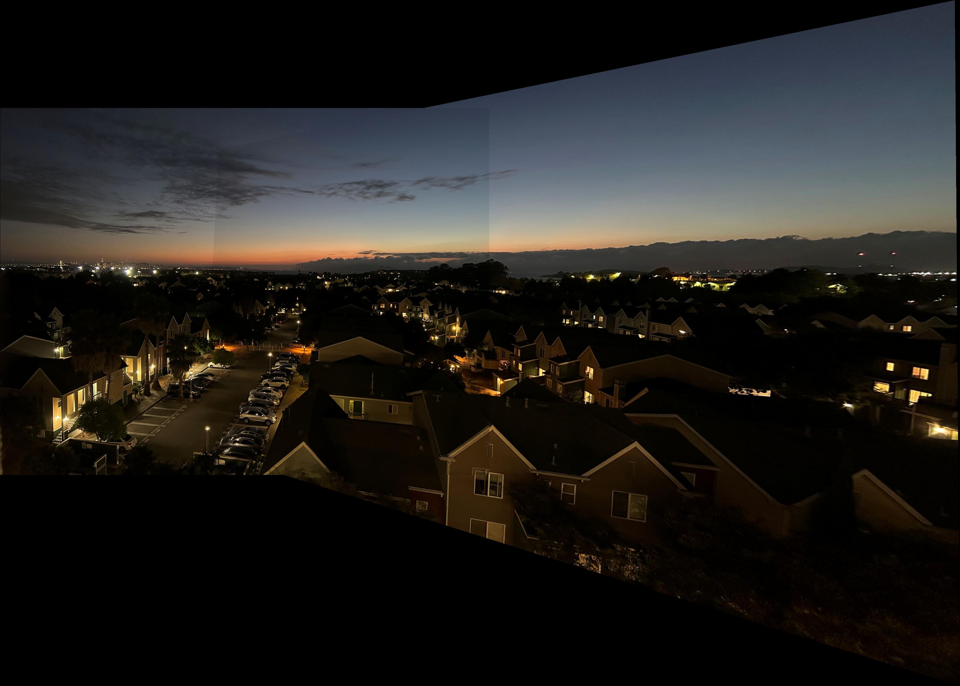
B.4 – RANSAC for Robust Homography & Mosaics

Using 4-point RANSAC, we estimate a homography from inlier matches, warp one image into the other’s frame, and blend to form a mosaic.

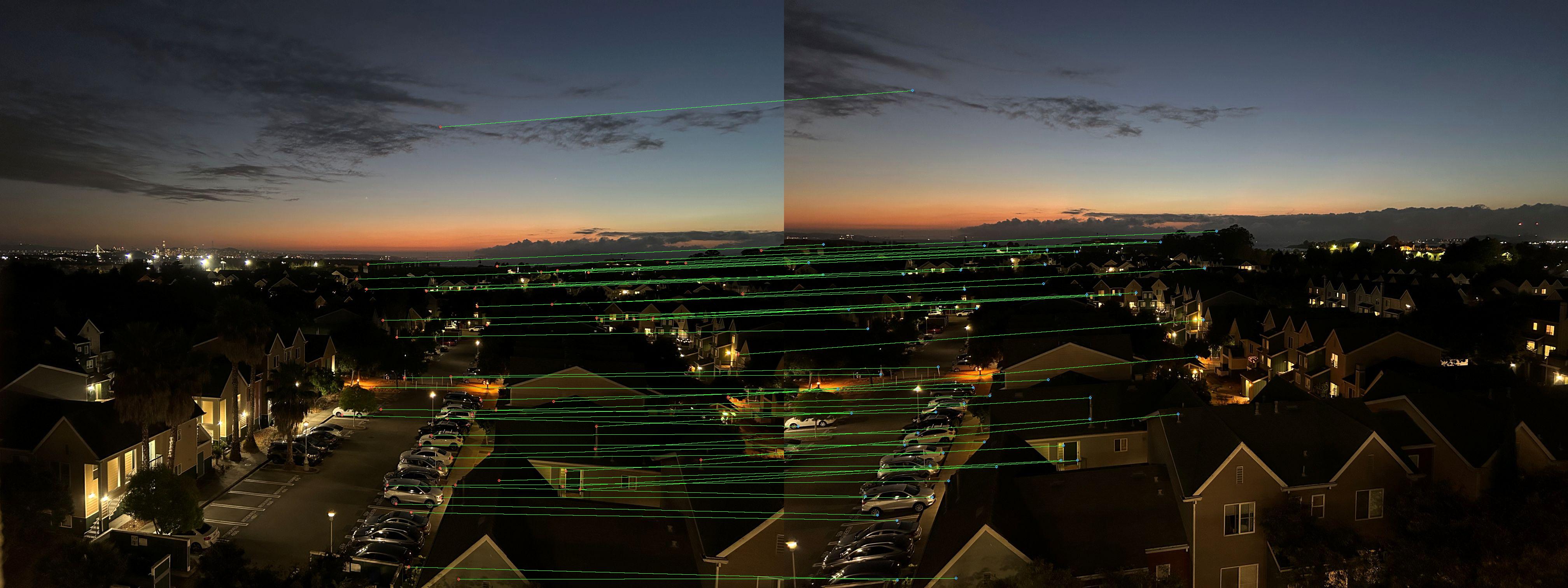
What is a homography? It’s a 3×3 matrix that maps points from one flat view to another (e.g., two photos of the same wall taken from different positions). With enough correct point pairs, we can estimate this matrix and use it to align entire images.

Why RANSAC? Some matches are wrong. RANSAC repeatedly picks 4 random pairs, computes a candidate homography, and counts how many matches agree (inliers). The candidate with the most inliers “wins”, and we refit using just those inliers for accuracy.

From math to pixels: Once we have the homography, we inverse‑warp the moving image into a shared canvas and blend overlaps with soft weights so seams fade away.

Implementation (RANSAC + inverse warp)

def ransac_fit_homography(src_xy: np.ndarray, dst_xy: np.ndarray, max_iters: int = ransac_max_iterations, eps: float = ransac_inlier_epsilon):
    best_inlier_mask = None
    best_homography = None
    count = src_xy.shape[0]
    if count < 4:
        return None, np.array([], dtype=bool)
    for _ in range(max_iters):
        sample_idx = np.random.choice(count, 4, replace=False)
        candidate = dlt_homography(src_xy[sample_idx], dst_xy[sample_idx])
        predicted = apply_homography_points(src_xy, candidate)
        error = np.sqrt(np.sum((predicted - dst_xy) ** 2, axis=1))
        inliers = error < eps
        if best_inlier_mask is None or np.count_nonzero(inliers) > np.count_nonzero(best_inlier_mask):
            best_inlier_mask = inliers
            best_homography = candidate
    if best_inlier_mask is not None and np.count_nonzero(best_inlier_mask) >= 4:
        best_homography = dlt_homography(src_xy[best_inlier_mask], dst_xy[best_inlier_mask])
    else:
        best_homography = None
        best_inlier_mask = np.zeros(count, dtype=bool)
    return best_homography, best_inlier_mask

def inverse_warp_to_canvas(src_image: np.ndarray, inverse_homography: np.ndarray, canvas_height: int, canvas_width: int, canvas_offset_xy: Tuple[int, int], mode: str = "bilinear"):
    offset_x, offset_y = canvas_offset_xy
    channels = src_image.shape[2] if src_image.ndim == 3 else 1
    canvas = np.zeros((canvas_height, canvas_width, channels), dtype=np.float32)
    alpha = np.zeros((canvas_height, canvas_width), dtype=np.float32)
    sampler = sample_bilinear if mode == "bilinear" else sample_nearest
    h0, h1, h2 = inverse_homography[0], inverse_homography[1], inverse_homography[2]
    for Y in range(canvas_height):
        for X in range(canvas_width):
            Xc, Yc = float(X), float(Y)
            w = h2[0] * (Xc - offset_x) + h2[1] * (Yc - offset_y) + h2[2]
            if abs(w) < 1e-12:
                continue
            x = (h0[0] * (Xc - offset_x) + h0[1] * (Yc - offset_y) + h0[2]) / w
            y = (h1[0] * (Xc - offset_x) + h1[1] * (Yc - offset_y) + h1[2]) / w
            value, ok = sampler(src_image, x, y)
            if ok:
                canvas[Y, X] = value
                alpha[Y, X] = 1.0
    return canvas, alpha

Walkthrough. ransac_fit_homography loops over random 4‑point samples to propose a homography via DLT, labels inliers by reprojection error < eps, and keeps the proposal with the largest consensus before refitting on all inliers. inverse_warp_to_canvas then maps every output pixel back into the source via the inverse homography and samples (bilinear by default); we also produce an alpha mask so overlapping images can be feather‑blended smoothly.

We randomly sample 4 correspondences to fit H (DLT), score inliers by reprojection error, keep the best consensus, refit on all inliers, then inverse-warp and feather-blend onto a common canvas.

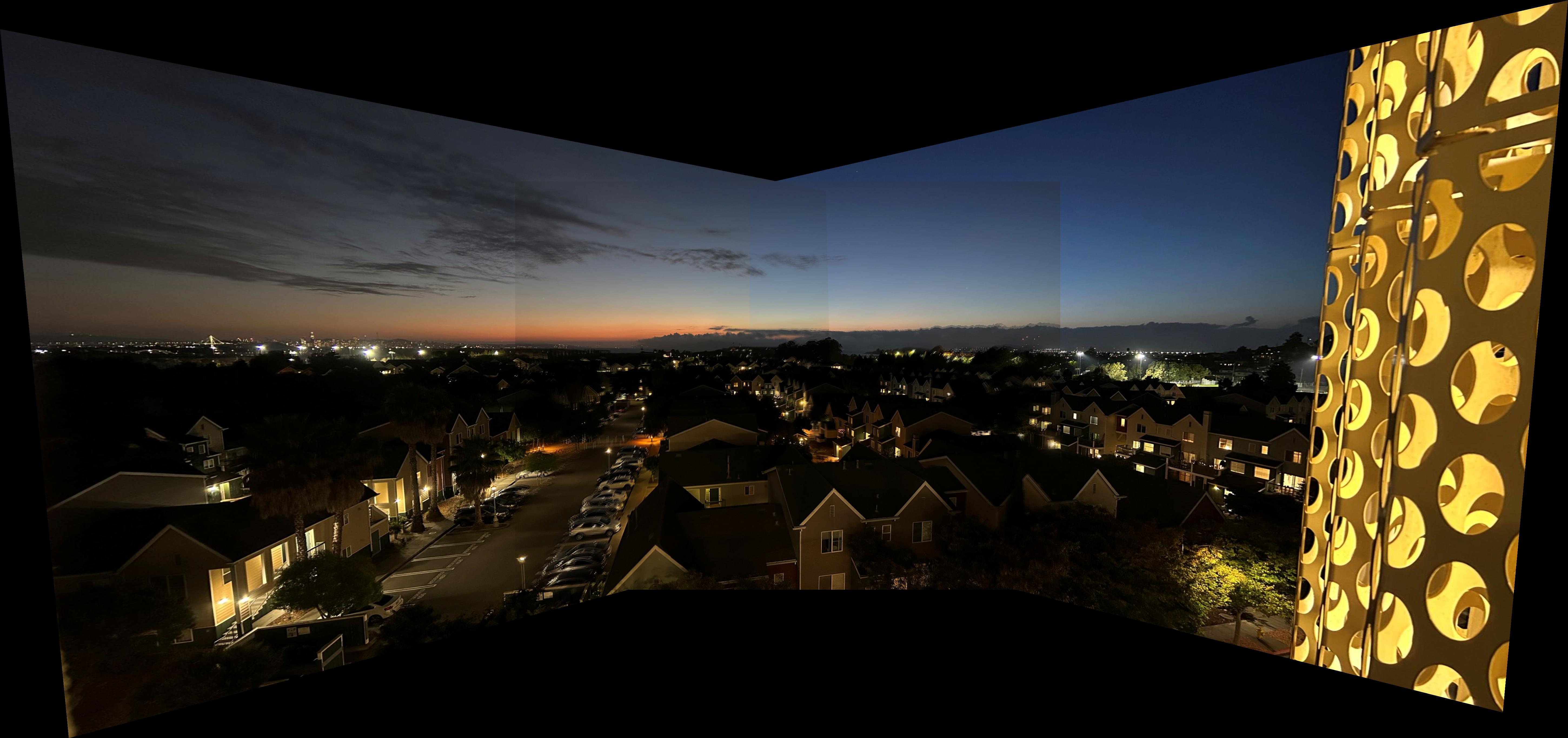
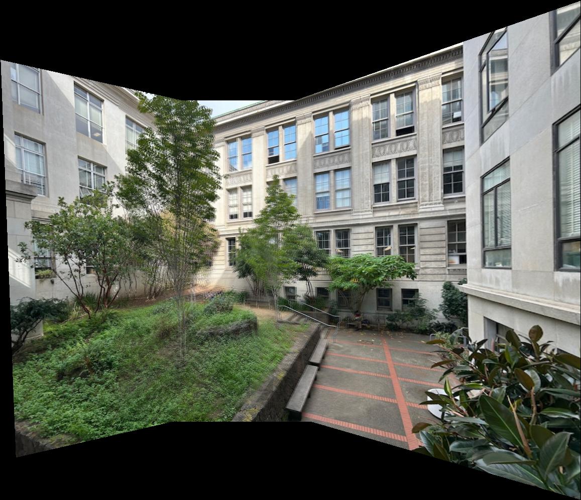
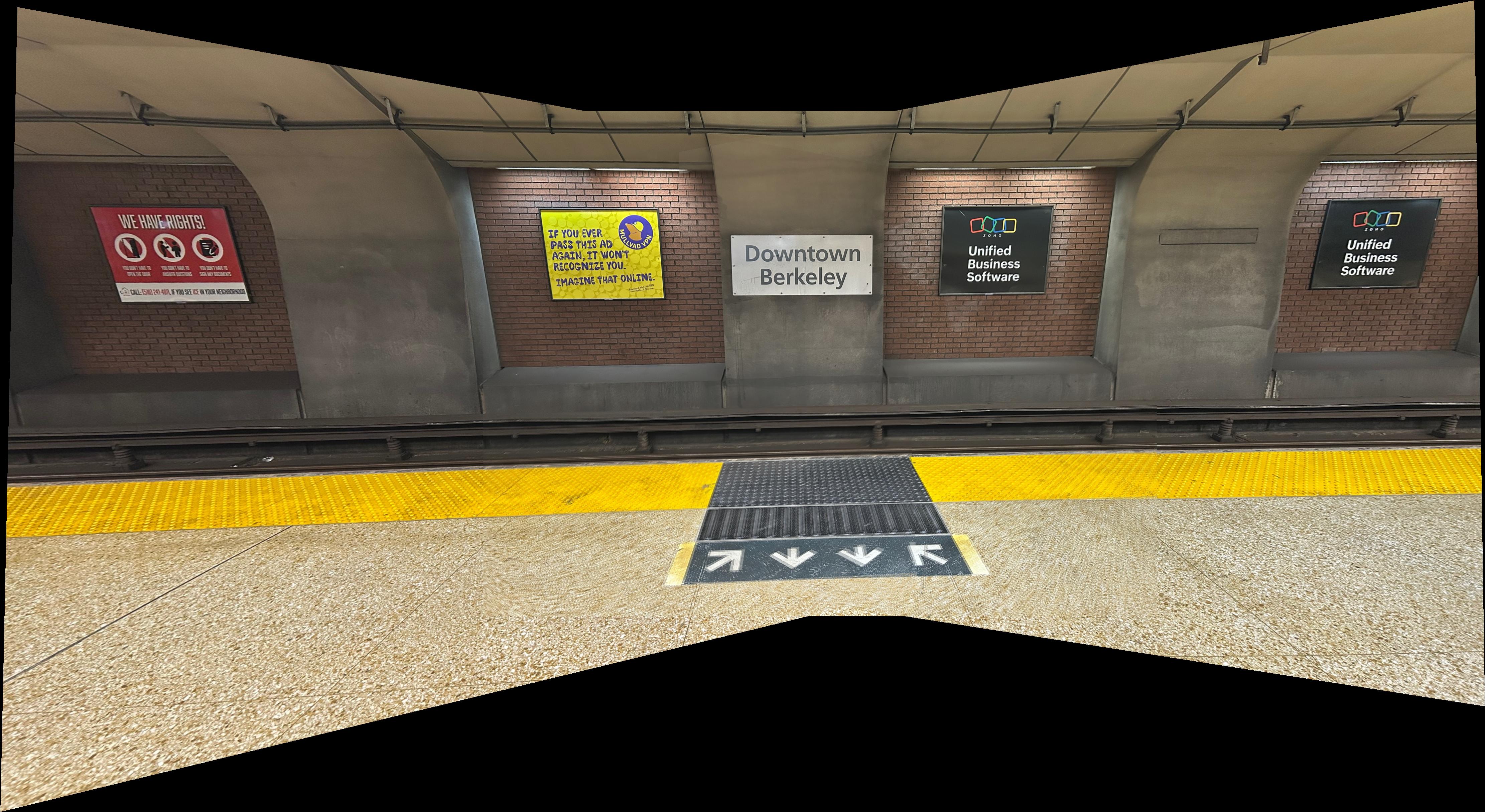
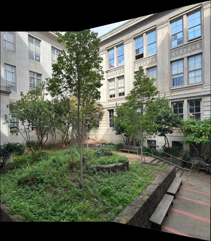
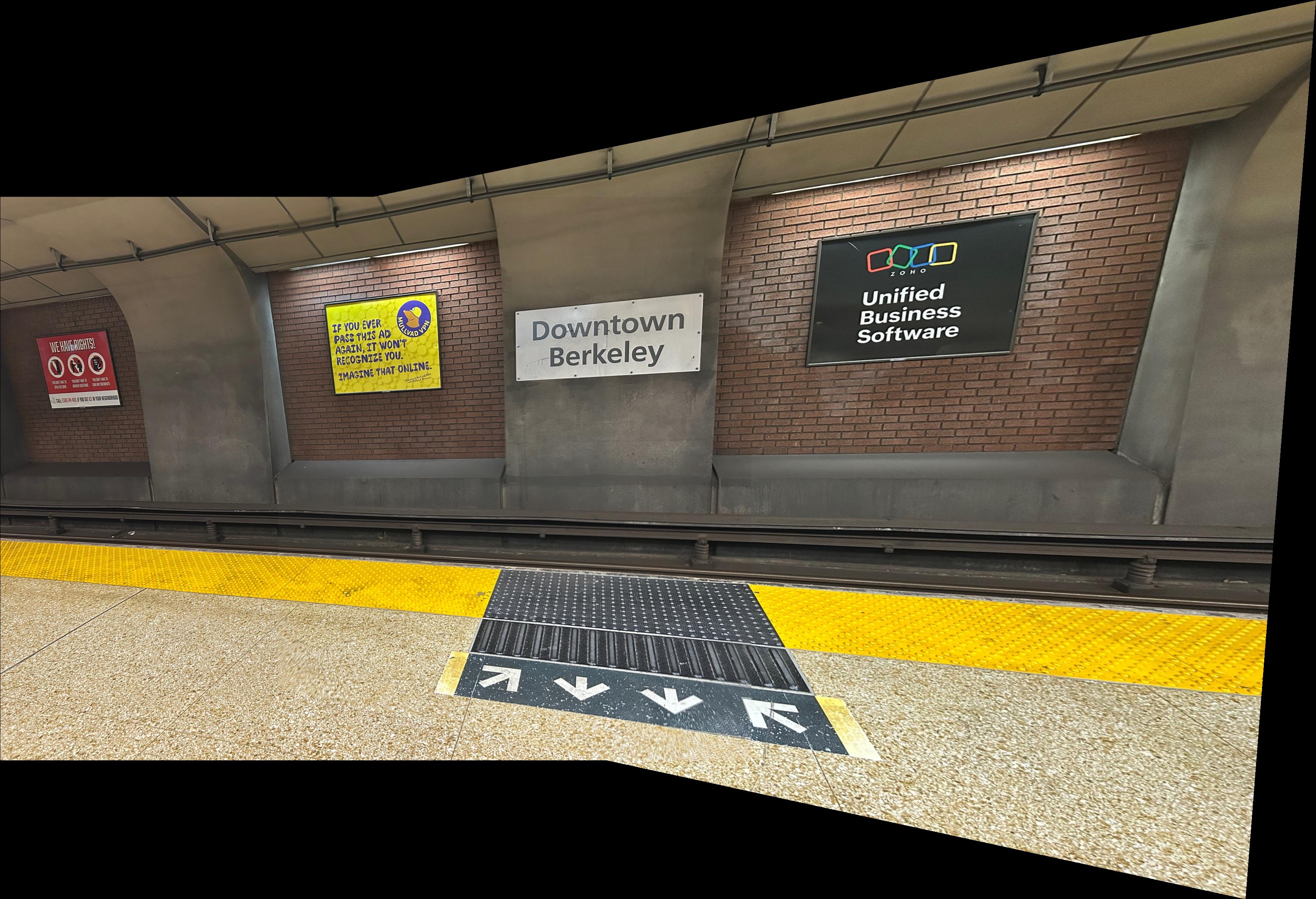
Results Gallery

Stitched panoramas from the full automatic pipeline (3B). Click to view full resolution.

Implementation Notes

Parameters (plain English). Harris threshold trades recall vs. noise; ANMS count controls spatial spread; Lowe ratio trades precision vs. recall; RANSAC epsilon is the inlier pixel error; iterations control robustness to outliers.

max_keypoints_after_anms = 750
harris_k_coeff = 0.04
harris_window_size = 3
harris_threshold_relative = 0.01
lowe_ratio_threshold = 0.7
ransac_max_iterations = 2000
ransac_inlier_epsilon = 3.0

References

• Brown, Szeliski, Winder. Multi-Image Matching using Multi-Scale Oriented Patches (MOPS).
• Harris & Stephens. A Combined Corner and Edge Detector.
• Lowe. Distinctive Image Features from Scale-Invariant Keypoints.

Last updated: —