Project 4 – Neural Radiance Fields (NeRF)
In this project I go from raw phone images of a small object to a fully learned, continuous 3D representation using Neural Radiance Fields (NeRF). The pipeline includes camera calibration and pose estimation, fitting a 2D neural field on an image, training a full NeRF on the classic Lego dataset, and finally learning a NeRF of my own object.
High-level Intuition
Rather than storing a 3D model as meshes or voxels, NeRF learns a continuous function that, given a point in 3D space
and a viewing direction, predicts color and density. By integrating these predictions along camera rays, we can render
realistic images from new viewpoints.
Part 0 – Calibrating Your Camera and Capturing a 3D Scan (0.1–0.4)
Before training any NeRF, we need accurate camera parameters. This part covers:
- 0.1 – Camera calibration with ArUco tags to recover intrinsics.
- 0.2 – Object capture with consistent lighting and distance.
- 0.3 – Pose estimation using Perspective-n-Point (PnP).
- 0.4 – Undistortion and dataset packaging into the NeRF-ready
.npzformat.
0.1 Camera Calibration with ArUco Tags
I printed an ArUco tag grid and captured 30–50 images from different angles while keeping the phone’s focal length fixed.
OpenCV detects the corners in 2D, which I associate with known 3D points on the flat tag. From those correspondences,
cv2.calibrateCamera estimates the camera intrinsics matrix and lens distortion.
import cv2, numpy as np

aruco_dict = cv2.aruco.getPredefinedDictionary(cv2.aruco.DICT_4X4_50)
aruco_params = cv2.aruco.DetectorParameters()

objpoints, imgpoints = [], []

def tag_corners_3d(tag_size_m=0.02):
    s = tag_size_m
    return np.array([
        [0.0, 0.0, 0.0],
        [s,   0.0, 0.0],
        [s,   s,   0.0],
        [0.0, s,   0.0],
    ], dtype=np.float32)

world_corners = tag_corners_3d()

for path in calibration_image_paths:
    img = cv2.imread(path)
    gray = cv2.cvtColor(img, cv2.COLOR_BGR2GRAY)

    corners, ids, _ = cv2.aruco.detectMarkers(gray, aruco_dict, parameters=aruco_params)
    if ids is None:
        continue

    img_corners = np.concatenate(corners, axis=0).reshape(-1, 2).astype(np.float32)
    imgpoints.append(img_corners)

    obj_corners = np.tile(world_corners, (len(ids), 1))
    objpoints.append(obj_corners)

ret, K, dist_coeffs, rvecs, tvecs = cv2.calibrateCamera(
    objpoints, imgpoints, gray.shape[::-1], None, None
)
Walkthrough
The goal here is to translate the visual pattern on the ArUco grid into numerical constraints the solver can use to infer the camera’s focal length and principal point.
- ArUco setup: I create the predefined 4×4 ArUco dictionary and detector parameters. This tells OpenCV which family of markers to look for.
- 3D tag geometry:
tag_corners_3dreturns the four corners of a square tag in meters. I treat the tag as lying on thez = 0plane. - Loop over images: For each calibration photo, I convert to grayscale and run
detectMarkers. If detection fails, I skip the image so the pipeline is robust. - Collect 2D points: I concatenate all detected corners into a single 2D array
img_corners, which holds pixel coordinates. - Collect 3D points: For every detected tag, I append a copy of the 3D tag corner coordinates to
objpoints, giving the solver many 3D–2D correspondences. - Calibration: Finally,
cv2.calibrateCameraestimatesK(intrinsics) anddist_coeffs(lens distortion). These are the foundations for all later pose and NeRF computations.
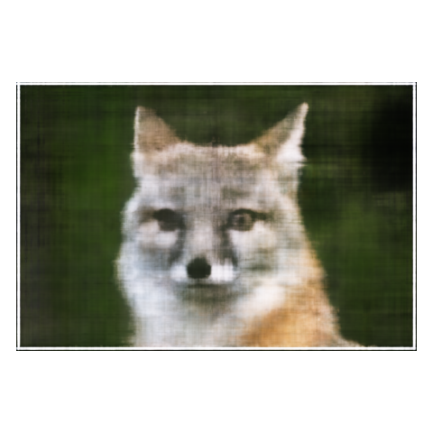
0.2 Object Capture
I chose a small object, placed a single ArUco tag on the table next to it, and captured 30–50 photos while moving the camera in an arc around the object. I tried to keep:
- Exposure roughly constant (no automatic brightness jumps).
- Blur minimal by holding the phone steady.
0.3 Pose Estimation and Viser Visualization
Using the intrinsics and distortion coefficients from calibration, I estimate the camera pose for each object image with
cv2.solvePnP. This gives me the camera’s rotation and translation relative to the tag, which I convert into a
camera-to-world matrix (c2w). I then visualize all the camera frustums in 3D using viser.
0.4 Undistortion & Dataset Packaging
NeRF assumes a simple pinhole camera model without lens distortion, so I undistort every image and crop valid pixels using
cv2.getOptimalNewCameraMatrix. I then build a .npz containing images and their corresponding
c2w matrices, split into train/val/test.
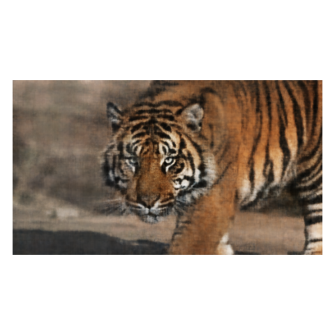
Part 1 – Fit a Neural Field to a 2D Image (1.1–1.4)
Before tackling full 3D NeRFs, I first train a 2D neural field that maps pixel coordinates to colors in a single image. This is an easier sandbox to understand positional encoding, MLP architecture, and training behavior.
1.1 Objective & Intuition
The neural field is a function F(u, v) → RGB that takes continuous, normalized pixel coordinates and outputs
the color at that point. Instead of storing the image as a grid of values, I store it as the weights of a neural network—
a kind of compressed, continuous representation.
1.2 Network & Positional Encoding
I use a small MLP with sinusoidal positional encoding (PE). PE expands coordinates into a higher-dimensional space using sines and cosines, enabling the network to capture fine details and edges.
import torch
import torch.nn as nn
import torch.nn.functional as F

class PosEnc(nn.Module):
    def __init__(self, num_freqs: int = 10):
        super().__init__()
        self.num_freqs = num_freqs

    def forward(self, x):
        encodings = [x]
        for i in range(self.num_freqs):
            freq = 2.0 ** i * torch.pi
            encodings.append(torch.sin(freq * x))
            encodings.append(torch.cos(freq * x))
        return torch.cat(encodings, dim=-1)


class NeuralField2D(nn.Module):
    def __init__(self, width=128, num_freqs=10):
        super().__init__()
        self.pe = PosEnc(num_freqs)
        in_dim = 2 + 2 * 2 * num_freqs

        layers = []
        hidden_dims = [width] * 4
        last_dim = in_dim
        for h in hidden_dims:
            layers.append(nn.Linear(last_dim, h))
            layers.append(nn.ReLU(inplace=True))
            last_dim = h

        self.mlp = nn.Sequential(*layers)
        self.out_layer = nn.Sequential(
            nn.Linear(last_dim, 3),
            nn.Sigmoid(),
        )

    def forward(self, uv):
        x = self.pe(uv)
        h = self.mlp(x)
        rgb = self.out_layer(h)
        return rgb
Walkthrough
This block defines the core 2D neural field model. It hides most of the math of “fitting a function to an image” inside a simple PyTorch module.
PosEnc: The positional encoding layer takes raw(u, v)coordinates in[0, 1]and builds a richer feature vector using sine and cosine at exponentially increasing frequencies. This lets the MLP represent both smooth regions and sharp edges.- Frequency loop: For each
i, I computefreq = 2^i · π. Applyingsin(freq · x)andcos(freq · x)at multiple frequencies effectively creates a Fourier-like basis over coordinates. - Input dimension: The MLP input has the original 2 coordinates plus
2*(sin, cos)*num_freqsvalues per coordinate. Concatenating all of these yields a high-dimensional input describing the position. - MLP architecture: I use 4 fully connected layers with ReLU activations. This is enough capacity to memorize a moderate-resolution image without being too slow.
- Output layer: The final
Linear → Sigmoidblock maps to three channels in[0, 1], which correspond directly to RGB values.
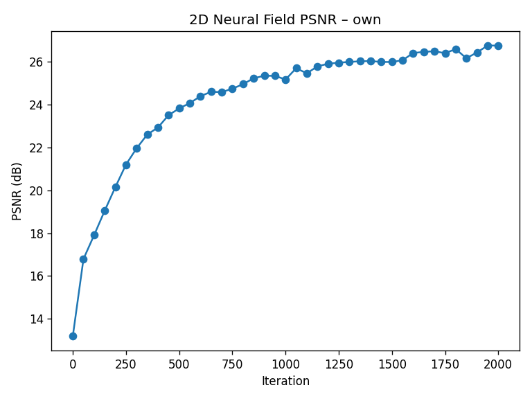
1.3 Training & PSNR
During training, I randomly sample 10k pixels at each iteration, feed their normalized coordinates into the network, and compare predicted colors against ground truth using mean squared error (MSE). I track reconstruction quality using PSNR (Peak Signal-to-Noise Ratio).
def train_2d_field(
    target_img,
    num_iters=2000,
    batch_size=8192,
    width=128,
    num_freqs=10,
    device=None,
):
    if device is None:
        device = torch.device("cuda" if torch.cuda.is_available() else "cpu")

    target = torch.as_tensor(target_img, dtype=torch.float32, device=device)
    target = target / 255.0 if target.max() > 1.0 else target
    H, W, _ = target.shape

    xs = torch.linspace(0.0, 1.0, W, device=device)
    ys = torch.linspace(0.0, 1.0, H, device=device)
    grid_x, grid_y = torch.meshgrid(xs, ys, indexing="xy")
    coords = torch.stack([grid_x, grid_y], dim=-1).view(-1, 2)
    colors = target.view(-1, 3)

    model = NeuralField2D(width=width, num_freqs=num_freqs).to(device)
    opt = torch.optim.Adam(model.parameters(), lr=1e-3)

    psnr_history = []

    for it in range(num_iters):
        idx = torch.randint(0, coords.shape[0], (batch_size,), device=device)
        uv = coords[idx]
        rgb_gt = colors[idx]

        rgb_pred = model(uv)
        loss = F.mse_loss(rgb_pred, rgb_gt)

        opt.zero_grad()
        loss.backward()
        opt.step()

        mse = loss.detach()
        psnr = -10.0 * torch.log10(mse)
        psnr_history.append(psnr.item())

    return model, psnr_history
Walkthrough
This training loop turns the static image into a dataset of coordinates and colors, then optimizes the MLP to regress from the former to the latter.
- Coordinate grid: I create a full grid of normalized
(u, v)coordinates and flatten it so each row corresponds to a pixel. - Targets: The target image is reshaped to match, so each coordinate has a matching RGB color.
- Mini-batches: At every iteration, I sample
batch_sizerandom pixels to improve convergence speed and generalization. - Optimization: I use Adam with a small learning rate and optimize MSE between predicted and target colors.
- PSNR tracking: I convert the MSE on each batch into PSNR and store it for plotting the learning curve.

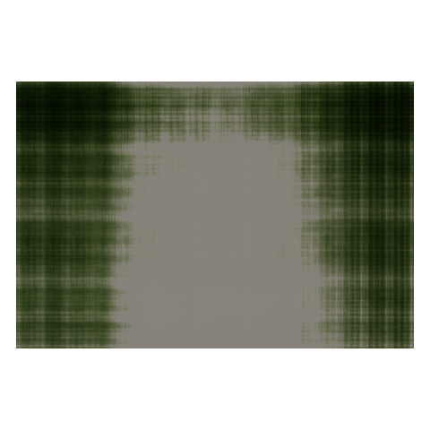
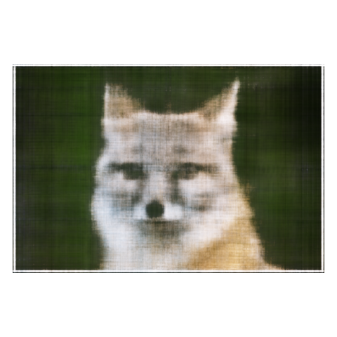


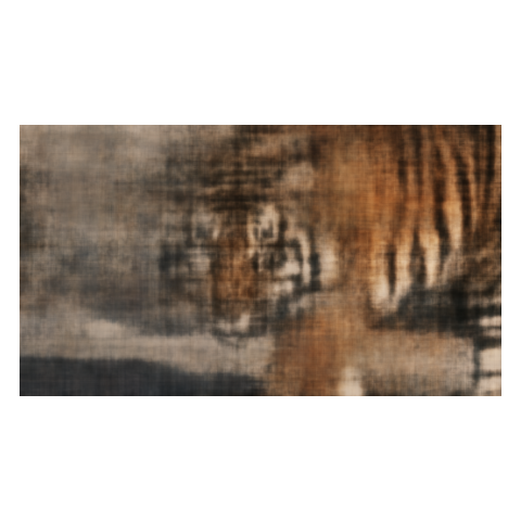
1.4 Hyperparameter Sweeps
I sweep over two key hyperparameters: the width of the MLP and the maximum PE frequency L. The following grid
shows how capacity and frequency content affect sharpness:


Takeaway
Positional encoding is what allows the MLP to represent crisp edges and small details, while width controls how much capacity
the network has to memorize complex textures. Together, they determine the trade-off between smoothness and fidelity.
Part 2 – Fit a Neural Radiance Field from Multi-view Images (2.1–2.5)
With 2D neural fields working, I move to the full 3D NeRF setup on the classic Lego dataset. Here the model takes 3D points and viewing directions as input and predicts both density and color, which are combined using volume rendering.
2.1 Rays from Cameras
I first convert pixel coordinates into 3D rays using the camera intrinsics and camera-to-world matrices. Each ray has an origin (camera center) and a direction in world space.
import torch

def pixel_to_camera(K, uv, depth=1.0):
    fx, fy = K[0, 0], K[1, 1]
    cx, cy = K[0, 2], K[1, 2]

    u, v = uv[..., 0], uv[..., 1]
    x = (u - cx) / fx * depth
    y = (v - cy) / fy * depth
    z = torch.full_like(x, depth)
    return torch.stack([x, y, z], dim=-1)


def pixel_to_ray(K, c2w, uv):
    depth = 1.0
    cam_pts = pixel_to_camera(K, uv, depth)

    R = c2w[:3, :3]
    t = c2w[:3, 3]
    world_pts = (R @ cam_pts.T).T + t

    ray_o = t.expand_as(world_pts)
    ray_d = world_pts - ray_o
    ray_d = ray_d / ray_d.norm(dim=-1, keepdim=True)
    return ray_o, ray_d
Walkthrough
This code bridges 2D image space and 3D world space, which is essential for NeRF: we must know which 3D line each pixel corresponds to.
pixel_to_camera: Uses the pinhole camera model: subtract the principal point(cx, cy), divide by focal lengths, and scale by depth. This “unprojects” a pixel into a 3D point at distance 1 along the camera’s optical axis.- Camera coordinates to world coordinates: Multiplying by
Rand addingteffectively rotates and translates points from the camera’s frame to the world frame. - Ray origin: The ray origin is just the camera center, which is
twhenc2wis camera-to-world. - Ray direction: I compute
world_pts - ray_oand normalize it to get a unit direction vector. - Batching: Everything is implemented in a vectorized way to efficiently handle many rays per training step.
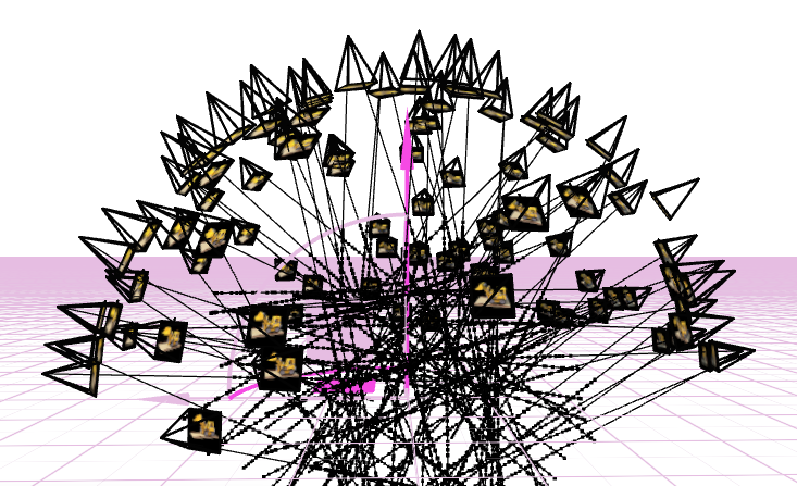
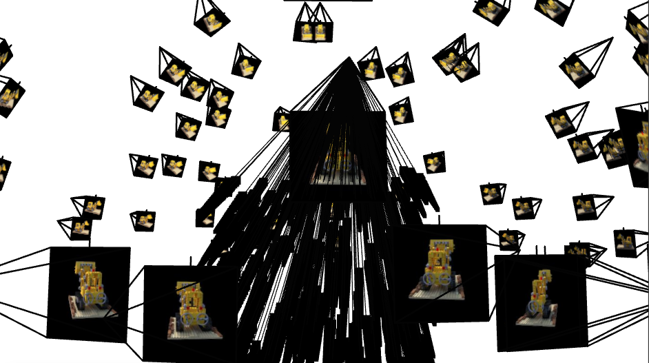
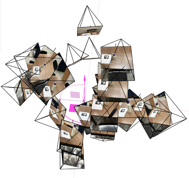
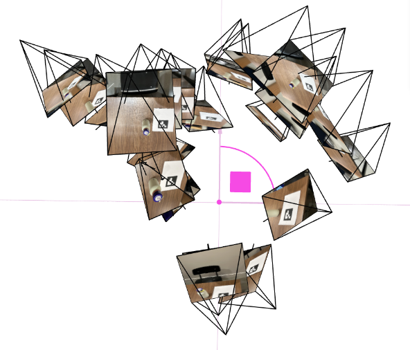
Viser validation visuals?
These 3D plots are a quick, visual “sanity check” that all upstream geometry is consistent before training NeRF. They confirm that
intrinsics (from calibration), undistortion, PnP poses, and my camera-to-world (c2w) convention agree with each other in a single,
real-world coordinate frame.
- Pose coherence: Camera frustums form a smooth arc around the object, with consistent “up” direction. Sudden jumps or twists usually mean a flipped axis or mixed conventions (
w2cvsc2w). - Scale & bounds: Distances between cameras and the tag/object look physically plausible, helping me pick reasonable
near/farranges for ray sampling. - Coverage: The orbit shows whether viewpoints sufficiently wrap the object (front, sides, some elevation). Sparse or clustered views predict holes/blur in the NeRF.
- Error spotting: Mis-undistortion, wrong principal point, or transposed rotations manifest immediately as crossed frustums, shears, or cameras pointing the wrong way.
How to read the plots
The pyramids are camera “cones” pointing where each photo looked. A clean ring with cones aimed at the same target implies consistent
poses. If cones diverge, flip, or intersect oddly, fix calibration/EXIF/pose code before training—otherwise the NeRF will try to
explain bad geometry with blurry density.
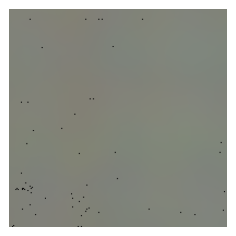
2.2 Sampling Points along Rays
For each ray, I sample a set of points between a near and far bound (2.0 and 6.0 for the Lego scene). During training, I add small random perturbations to encourage the model to cover the entire interval and avoid overfitting to a fixed grid.
def sample_along_rays(rays_o, rays_d, n_samples=64, near=2.0, far=6.0, perturb=True):
    B = rays_o.shape[0]
    t_vals = torch.linspace(near, far, n_samples, device=rays_o.device)
    t_vals = t_vals.expand(B, n_samples)

    if perturb:
        mids = 0.5 * (t_vals[:, :-1] + t_vals[:, 1:])
        widths = t_vals[:, 1:] - t_vals[:, :-1]
        noise = (torch.rand_like(mids) - 0.5) * widths
        t_vals = torch.cat([mids + noise, t_vals[:, -1:]], dim=-1)

    points = rays_o[..., None, :] + rays_d[..., None, :] * t_vals[..., None]
    return points, t_vals
Walkthrough
NeRF is essentially integrating along each ray, so we approximate that integral by sampling discrete points.
- Base sampling:
torch.linspace(near, far, n_samples)gives evenly spaced depths along the ray. Each ray shares the same initial sample depths. - Perturbation: To avoid aliasing artifacts, I jitter the sample positions inside each interval. This is similar to anti-aliasing in rendering and helps cover the continuous volume more uniformly.
- 3D point computation: The formula
rays_o + rays_d * tgives the 3D point at distancetalong the ray. - Shape: The result
pointshas shape[B, N, 3], which is convenient for feeding into the NeRF MLP.
2.3 NeRF Network Architecture
The NeRF network takes in 3D points and viewing directions, applies separate positional encodings, and outputs a density (scalar) and an RGB color conditioned on direction.
class NeRF(nn.Module):
    def __init__(self, pos_freqs=10, dir_freqs=4, width=256):
        super().__init__()
        self.pos_pe = PosEnc(pos_freqs)
        self.dir_pe = PosEnc(dir_freqs)

        pos_dim = 3 + 2 * 3 * pos_freqs
        dir_dim = 3 + 2 * 3 * dir_freqs

        self.fc_pos = nn.Sequential(
            nn.Linear(pos_dim, width), nn.ReLU(True),
            nn.Linear(width, width),   nn.ReLU(True),
            nn.Linear(width, width),   nn.ReLU(True),
            nn.Linear(width, width),   nn.ReLU(True),
        )

        self.fc_pos2 = nn.Sequential(
            nn.Linear(width + pos_dim, width),
            nn.ReLU(True),
        )

        self.sigma_head = nn.Sequential(
            nn.Linear(width, 1),
            nn.ReLU(),
        )

        self.fc_feat = nn.Linear(width, width)
        self.fc_rgb = nn.Sequential(
            nn.Linear(width + dir_dim, width // 2),
            nn.ReLU(True),
            nn.Linear(width // 2, 3),
            nn.Sigmoid(),
        )

    def forward(self, x, d):
        B, N, _ = x.shape

        x_enc = self.pos_pe(x.view(-1, 3))
        h = self.fc_pos(x_enc)
        h = self.fc_pos2(torch.cat([h, x_enc], dim=-1))

        sigma = self.sigma_head(h)

        d_enc = self.dir_pe(d.view(-1, 3))
        feat = self.fc_feat(h)
        h_color = torch.cat([feat, d_enc], dim=-1)
        rgb = self.fc_rgb(h_color)

        sigma = sigma.view(B, N, 1)
        rgb = rgb.view(B, N, 3)
        return sigma, rgb
Walkthrough
This is the core of the NeRF: a network that translates coordinates and directions into physical quantities used by the volume renderer.
- Separate encodings: I encode
x(3D position) andd(view direction) separately. Positions usually require higher frequencies than directions. - Position branch: The encoded position goes through several fully connected layers with ReLU, forming a deep feature representation of local geometry.
- Skip connection: Concatenating
hwithx_encmid-way helps the network keep track of the original spatial location and improves training stability. - Density head: The
sigma_headpredicts a non-negative density through a ReLU, representing how much light is absorbed or scattered at each point. - Color head: The color branch takes both the feature vector from geometry and the encoded viewing direction. This allows the network to model view-dependent effects like specular highlights.
- Reshaping: After computing
sigmaandrgbforB·Npoints, I reshape them back to[B, N, ·]so they line up with the sampled points along each ray.
2.4 Volume Rendering
To render a pixel, I convert densities to opacities and integrate colors along the ray using the NeRF volume rendering equation. In discrete form, each sample contributes:
color = Σ Ti · αi · ci, where Ti is the accumulated transmittance up to sample i,
and αi = 1 - exp(-σi Δt) is the opacity.
def volume_render(sigmas, rgbs, t_vals):
    B, N, _ = sigmas.shape
    deltas = t_vals[:, 1:] - t_vals[:, :-1]
    deltas = torch.cat([deltas, deltas[:, -1:]], dim=-1)

    alpha = 1.0 - torch.exp(-sigmas.squeeze(-1) * deltas)

    accum = torch.cumsum(-sigmas.squeeze(-1) * deltas, dim=-1)
    T = torch.exp(torch.cat([torch.zeros(B, 1, device=sigmas.device), accum[:, :-1]], dim=-1))

    weights = T * alpha
    rgb_map = (weights[..., None] * rgbs).sum(dim=1)
    return rgb_map
Walkthrough
This function numerically approximates the continuous volume rendering integral using the discrete samples produced earlier.
- Δt computation:
deltasstores the distance between consecutive samples along the ray. The last interval is copied from the previous one. - Opacity α: I convert densities into opacities using
α = 1 − exp(−σ Δt). This comes from the Beer–Lambert law of light attenuation. - Transmittance T: The cumulative sum of
−σ Δtgives the accumulated optical thickness. Exponentiating yields transmittance: the probability that light survives from the ray origin to the current sample. - Weights: Each sample’s contribution is
T · α, meaning “the ray reaches this point and then terminates here.” - Final color: I multiply each sample’s color by its weight and sum along the ray dimension, producing one RGB value per ray.
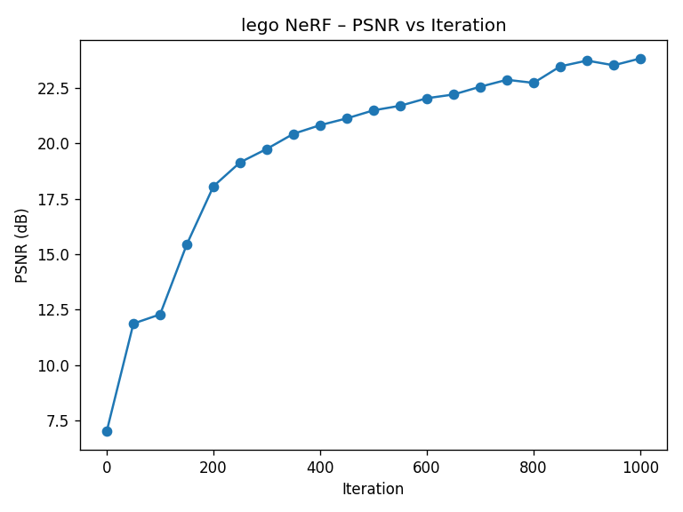
2.5 Training & Results on the Lego Scene
I train NeRF on the Lego dataset using Adam (learning rate 5e-4) with 10k rays per iteration. The validation PSNR reaches above the 23 dB target within 1000 gradient steps.
def train_nerf_lego(
    images,
    c2ws,
    focal,
    num_iters=1000,
    rays_per_batch=10000,
    n_samples=64,
    near=2.0,
    far=6.0,
    device=None,
):
    if device is None:
        device = torch.device("cuda" if torch.cuda.is_available() else "cpu")

    imgs = torch.as_tensor(images, dtype=torch.float32, device=device)
    imgs = imgs / 255.0 if imgs.max() > 1.0 else imgs
    N, H, W, _ = imgs.shape
    imgs_flat = imgs.view(-1, 3)

    K = torch.tensor(
        [[focal, 0.0, W / 2.0],
         [0.0,   focal, H / 2.0],
         [0.0,   0.0,   1.0]],
        dtype=torch.float32,
        device=device,
    )

    ix, iy = torch.meshgrid(
        torch.arange(W, device=device),
        torch.arange(H, device=device),
        indexing="xy"
    )
    uv = torch.stack([ix + 0.5, iy + 0.5], dim=-1).view(-1, 2)

    rays_o_all = []
    rays_d_all = []
    for c2w in c2ws:
        c2w_t = torch.as_tensor(c2w, dtype=torch.float32, device=device)
        ray_o, ray_d = pixel_to_ray(K, c2w_t, uv)
        rays_o_all.append(ray_o)
        rays_d_all.append(ray_d)

    rays_o_all = torch.cat(rays_o_all, dim=0)
    rays_d_all = torch.cat(rays_d_all, dim=0)

    model = NeRF().to(device)
    opt = torch.optim.Adam(model.parameters(), lr=5e-4)

    psnr_history = []

    for it in range(num_iters):
        idx = torch.randint(0, rays_o_all.shape[0], (rays_per_batch,), device=device)
        rays_o = rays_o_all[idx]
        rays_d = rays_d_all[idx]
        target = imgs_flat[idx]

        pts, t_vals = sample_along_rays(rays_o, rays_d, n_samples, near, far, perturb=True)
        sigmas, rgbs = model(
            pts,
            rays_d[..., None, :].expand_as(pts),
        )
        rgb_map = volume_render(sigmas, rgbs, t_vals)

        loss = F.mse_loss(rgb_map, target)

        opt.zero_grad()
        loss.backward()
        opt.step()

        mse = loss.detach()
        psnr = -10.0 * torch.log10(mse)
        psnr_history.append(psnr.item())

    return model, psnr_history
Walkthrough
This training loop ties together rays, samples, the NeRF MLP, and the volume renderer into a single optimization problem.
- Ray precomputation: I build a pinhole intrinsics matrix from the Lego focal length, then unproject every pixel of every view into a world-space ray using
pixel_to_ray. - Dataset flattening: All ray origins, ray directions, and RGB colors are flattened so each index corresponds to a single ray–pixel pair.
- Mini-batch sampling: At each iteration I randomly choose
rays_per_batchrays, sample 3D points along them, and query the NeRF network. - Rendering:
volume_renderintegrates densities and colors along each ray to produce a batch of predicted pixel colors. - Loss + PSNR: I minimize MSE between rendered colors and ground-truth pixels using Adam, and track PSNR to monitor how quickly the model is fitting the multi-view data.
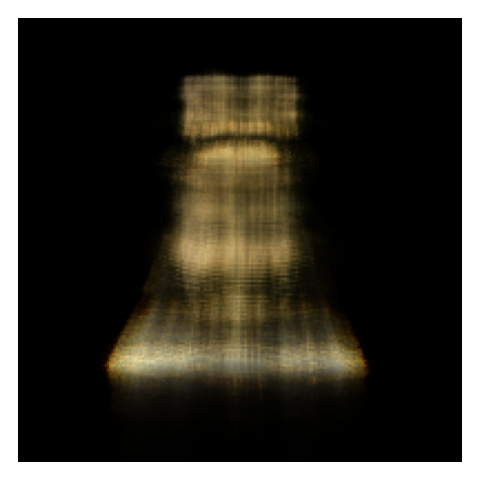
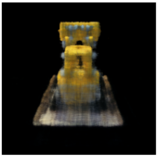
2.5.1 Spherical Novel-View Rendering
To demonstrate true 3D understanding, I render novel views of the Lego scene from a spherical trajectory around the object. The NeRF is never explicitly told about these views; it synthesizes them from the learned radiance field.
Takeaway
The Lego experiment demonstrates that NeRF can recover a coherent 3D representation purely from multiple images and camera
poses, without any explicit 3D supervision. Everything emerges from minimizing reconstruction error across views.
Part 2.6 – Training with My Own Object Data (2.6.1–2.6.4)
Finally, I apply the entire NeRF pipeline to the dataset I captured in Part 0, training a NeRF that can synthesize novel views of my own object.
2.6.1 Dataset & Preprocessing
I use the undistorted images and c2w matrices produced earlier and package them into
images_train, images_val, c2ws_train, and c2ws_val. I slightly adjust
near/far bounds and number of samples to match the physical size of my scene (e.g., near ≈ 0.02,
far ≈ 0.5, 64 samples per ray).
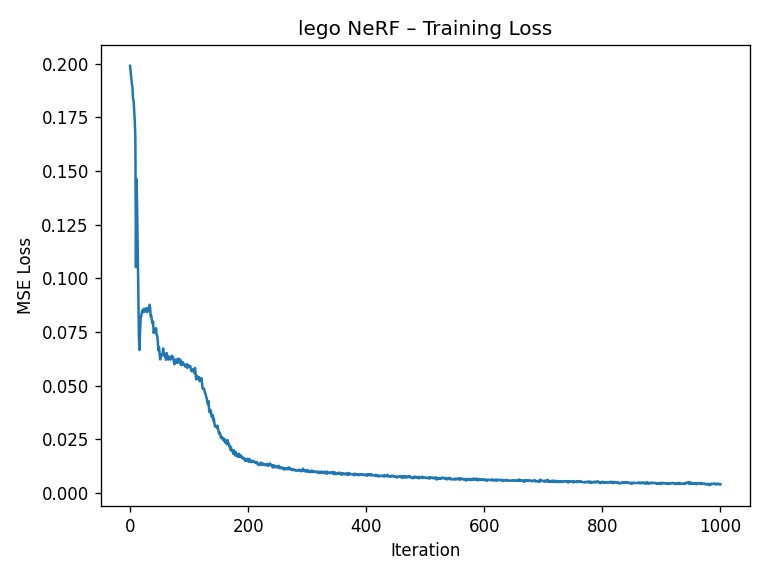
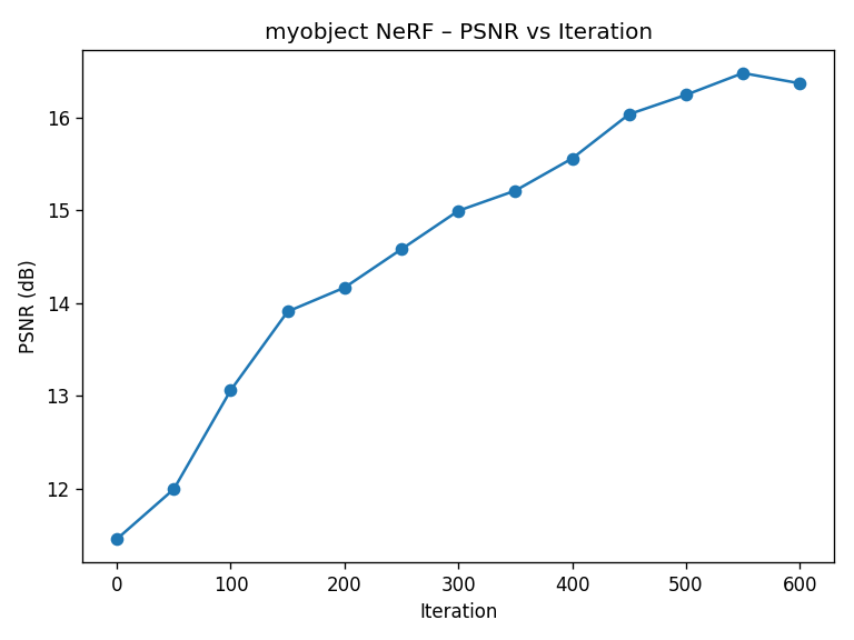
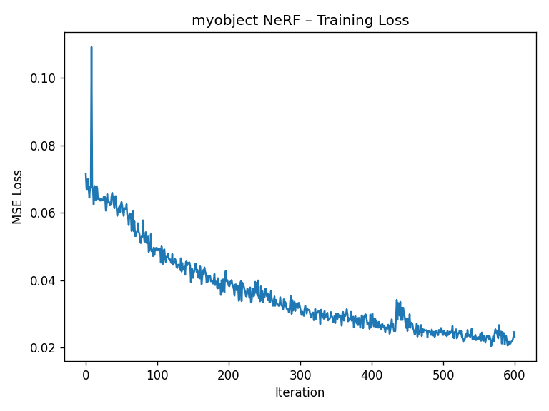
2.6.2 Training Behavior
Training behavior is similar to Lego but a bit more sensitive to hyperparameters, since my capture is less “perfect” than the synthetic dataset. The loss curve below shows the training loss decreasing over time.
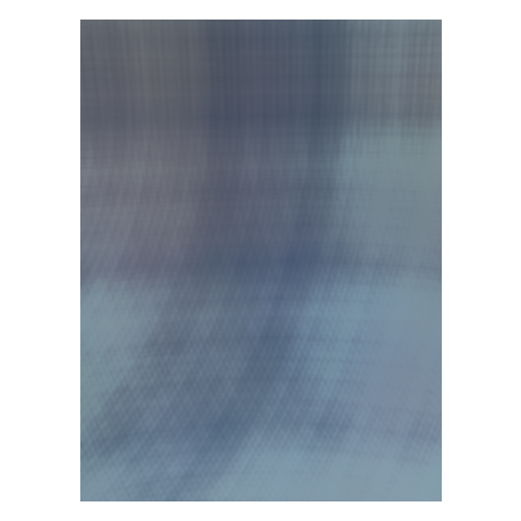

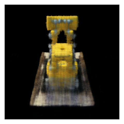
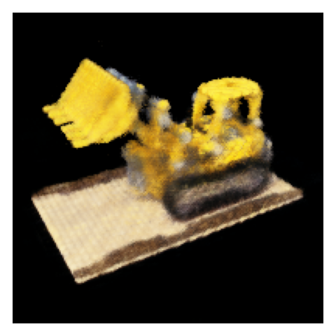
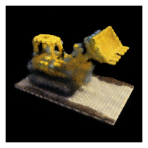
2.6.3 Novel View Animation
I synthesize a small orbiting camera path around the object by creating new c2w matrices that place the camera
on a circle, always looking at the origin. For each frame, I render an image using the trained NeRF and combine them into a GIF.


2.6.4 Reflection
Compared to the Lego scene, my own data is noisier, less uniformly lit, and has fewer views. Nonetheless, NeRF is able to reconstruct a coherent 3D model that produces convincing novel views. This highlights both the power and fragility of the method: it can interpolate impressively, but is sensitive to calibration quality, coverage, and exposure consistency.
Implementation Notes & Pitfalls
This section summarizes key parameter choices and practical issues I encountered while implementing NeRF from scratch.
- Batch size: I used around 10k rays per iteration for Lego. Larger batches stabilize training but increase GPU memory usage.
- Near/Far bounds: Getting these wrong either wastes samples (too wide) or chops off geometry (too tight).
For my object I tuned
nearandfarby visualizing depth and trying a few ranges. - Positional encoding frequencies: Very high frequencies can cause ringing artifacts if the network or data
can’t support them. I found
pos_freqs≈10,dir_freqs≈4to be a good balance. - Learning rate: For Lego I used
5e-4with Adam. Higher learning rates converged faster but risked oscillations in PSNR. - Data quality: Slight miscalibration (especially in intrinsics) can produce subtle ghosting in the final NeRF. Carefully checking the Viser camera cloud was essential before committing to long training runs.
- Debugging strategy: I verified each stage (ray directions, sampling locations, volume rendering) with small, synthetic tests before combining them. This helped isolate bugs that would otherwise manifest as “blurry renderings.”
Lessons Learned
NeRF looks intimidating because of the integral in the volume rendering equation, but in code it’s mostly linear algebra and
exponentials. The hard part isn’t the math—it’s keeping every coordinate system, normalization, and range consistent across
the entire pipeline.
References
- Mildenhall et al., NeRF: Representing Scenes as Neural Radiance Fields for View Synthesis, ECCV 2020.
- CS180: Intro to Computer Vision and Computational Photography – Project 4 spec and starter code.
- OpenCV documentation: camera calibration, ArUco detection, and PnP pose estimation.
- PyTorch documentation for building and training neural networks on GPU.