Overview

Both parts solve the same core problem: how do we turn random noise into a meaningful image?

Intuition Part A is like learning to drive by using a powerful self-driving car but understanding the steering wheel (the sampling loop). Part B is building the engine: the UNet learns what “denoise” means from scratch, then we teach it a smooth path from noise to digits.

Part A (Project 5A) · The Power of Diffusion Models

This section preserves the original Project 5A structure and results, but labels each subsection with an A prefix.

A · Results

Required output images first, then each subsection explains how the result was produced.

A0 · Text-to-Image Sampling

Goal: pick 3 creative prompts, generate images, and compare at least 2 inference-step settings to show the quality tradeoff.

Takeaway More inference steps usually improves detail and coherence, but costs time. The “best” step count depends on whether you want speed or polish.

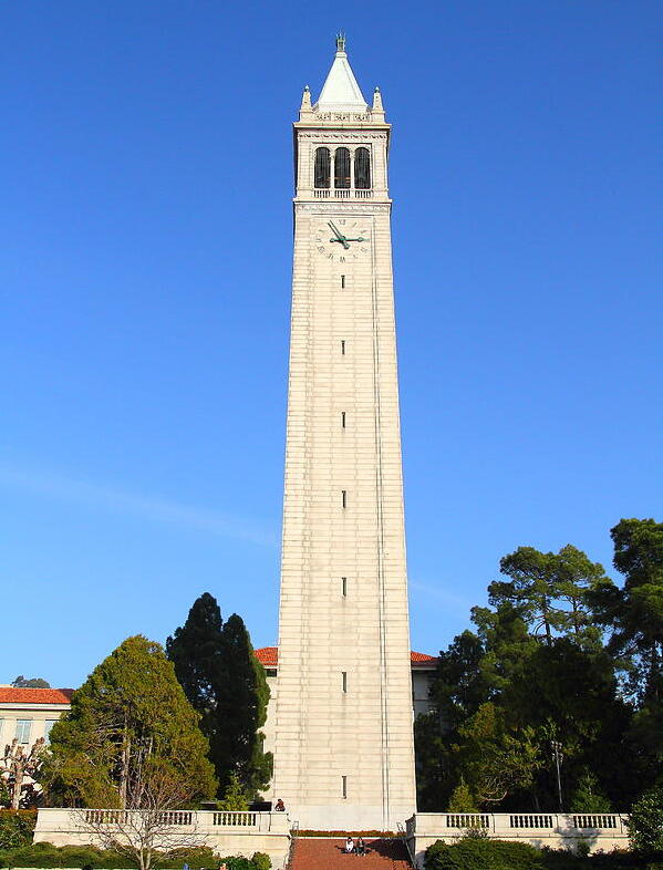
A1.1 · Forward Diffusion (Add Noise)

Goal: start with a clean image (Campanile), and show what it looks like after adding noise at three different timesteps: t=250, 500, 750.

# Forward process: x_t = sqrt(alpha_bar[t]) * x_0 + sqrt(1 - alpha_bar[t]) * eps
def noisy_im_forward(x0, t, alphas_cumprod):
    # Sample Gaussian noise with same shape as image
    eps = torch.randn_like(x0)
    alpha_bar_t = alphas_cumprod[t]
    xt = torch.sqrt(alpha_bar_t) * x0 + torch.sqrt(1 - alpha_bar_t) * eps
    return xt, eps
      

Walkthrough: We simulate what the diffusion training data looks like. First we draw random noise eps. Then we mix the clean image x0 with that noise using a schedule value alpha_bar_t. When t is small, alpha_bar_t is closer to 1 so the image is mostly intact. When t is large, alpha_bar_t shrinks and the image becomes dominated by noise. This “controlled corruption” is the foundation for both denoising and editing later.

A1.2 · Classical Denoising (Gaussian Blur)

Goal: try to “denoise” the noisy images using a simple baseline (Gaussian blur) and show the best result for each timestep.

# Classical baseline: blur removes high-frequency noise, but also removes real detail
def gaussian_denoise(xt, kernel_size=33, sigma=2.0):
    return torchvision.transforms.functional.gaussian_blur(
        xt, kernel_size=[kernel_size, kernel_size], sigma=[sigma, sigma]
    )
      

Walkthrough: Gaussian blur is a simple filter that smooths an image by averaging nearby pixels. It often reduces “speckle” noise because noise changes rapidly from pixel to pixel. But it also destroys real edges and textures (which are also high-frequency content), so it’s a useful baseline: if the diffusion model beats this, we know it’s doing something smarter than smoothing.

A1.3 · One-Step Denoising (Pretrained UNet)

Goal: use the pretrained denoiser to predict the noise in each noisy image and remove it once.

# One-step: predict noise with UNet, then estimate x0 from xt
def one_step_denoise(xt, t, prompt_embeds, alphas_cumprod):
    model_out = stage_1.unet(xt, t, encoder_hidden_states=prompt_embeds, return_dict=False)[0]
    # DeepFloyd predicts (noise, variance); split by channel count
    noise_est, _ = torch.split(model_out, xt.shape[1], dim=1)
    alpha_bar_t = alphas_cumprod[t]
    x0_est = (xt - torch.sqrt(1 - alpha_bar_t) * noise_est) / torch.sqrt(alpha_bar_t)
    return x0_est
      

Walkthrough: The UNet is a neural network trained to look at a noisy image xt plus a timestep t and answer: “what noise was added to get here?” If we know the noise, we can algebraically rearrange the forward equation to estimate the original clean image x0. This is only one step, so it helps, but it’s not perfect. The real power comes from repeating this logic many times (next section).

A1.4 · Iterative Denoising (Sampling Loop)

Goal: implement the actual iterative loop: take a noisy image and gradually denoise it over a sequence of timesteps.

# Iterative denoising loop (core sampling idea)
def iterative_denoise(x_start, timesteps, prompt_embeds, alphas_cumprod):
    x = x_start
    with torch.no_grad():
        for i in range(len(timesteps) - 1):
            t = timesteps[i]
            t_prev = timesteps[i + 1]

            model_out = stage_1.unet(x, t, encoder_hidden_states=prompt_embeds, return_dict=False)[0]
            noise_est, var_est = torch.split(model_out, x.shape[1], dim=1)

            alpha_bar_t = alphas_cumprod[t]
            alpha_bar_prev = alphas_cumprod[t_prev]

            # Estimate x0 (clean) at this step
            x0_est = (x - torch.sqrt(1 - alpha_bar_t) * noise_est) / torch.sqrt(alpha_bar_t)

            # Step to the previous timestep (less noise)
            x = torch.sqrt(alpha_bar_prev) * x0_est + torch.sqrt(1 - alpha_bar_prev) * noise_est
    return x
      

Walkthrough: This is the heart of diffusion. We begin at a noisy image x_start. At each timestep t, the UNet predicts the noise. From that, we estimate what the clean image would be (x0_est). Then we “rewind the clock” to a slightly less noisy timestep t_prev by recombining the clean estimate with the noise estimate. Repeating this many times is what turns noise into structure.

Comparison

A1.5 · Diffusion Sampling (from Random Noise)

Goal: start from pure random noise and run the iterative denoise loop to generate images.

Why it looks weak Without CFG, prompts influence the generation less strongly, so samples can look generic or off-topic. CFG fixes this next.

A1.6 · Classifier-Free Guidance (CFG)

Goal: denoise twice each step: once with the prompt, once with an “empty” prompt, then combine them to strengthen conditioning.

# CFG: eps = eps_uncond + scale * (eps_cond - eps_uncond)
def cfg_noise(x, t, prompt_embeds, uncond_prompt_embeds, scale=7):
    cond_out = stage_1.unet(x, t, encoder_hidden_states=prompt_embeds, return_dict=False)[0]
    uncond_out = stage_1.unet(x, t, encoder_hidden_states=uncond_prompt_embeds, return_dict=False)[0]
    eps_c, _ = torch.split(cond_out, x.shape[1], dim=1)
    eps_u, _ = torch.split(uncond_out, x.shape[1], dim=1)
    return eps_u + scale * (eps_c - eps_u)
      

Walkthrough: Think of eps_uncond as “what the model would do if you said nothing” and eps_cond as “what the model would do given your prompt.” CFG pushes the generation away from the unconditional direction and toward the prompt direction. The scale controls how strong that push is: higher gives more prompt adherence, but too high can make artifacts.

A1.7 · Image-to-Image Translation (SDEdit-style)

Goal: start from a real image, add noise, then denoise with CFG so the result stays “close” to the original while becoming more “diffusion-realistic.” We show a progression across noise levels [1, 3, 5, 7, 10, 20].

Intuition More starting noise gives the model more freedom to “rewrite” the image. Less noise preserves details but changes less.

Campanile Edit

My Own Image 1 Edit

My Own Image 2 Edit

A1.7.1 · Image-to-Image Translation Web and Hand-drawn Images

Web Image Edit

Handrawn Image 1 Edit

Handrawn Image 2 Edit

A1.7.2 · Inpainting

Goal: regenerate only a masked region while keeping the rest of the image locked to the original.

# Inpainting loop: after each denoise step, force unmasked pixels to match the original (with correct noise level)
def inpaint(x_orig, mask, timesteps, prompt_embeds, uncond_prompt_embeds, alphas_cumprod, scale=7):
    x = torch.randn_like(x_orig).half().to(x_orig.device)
    mask = mask.to(device=x.device, dtype=x.dtype)

    with torch.no_grad():
        for i in range(len(timesteps) - 1):
            t = timesteps[i]
            t_prev = timesteps[i + 1]

            eps = cfg_noise(x, t, prompt_embeds, uncond_prompt_embeds, scale=scale)

            alpha_bar_t = alphas_cumprod[t]
            alpha_bar_prev = alphas_cumprod[t_prev]

            x0_est = (x - torch.sqrt(1 - alpha_bar_t) * eps) / torch.sqrt(alpha_bar_t)
            x = torch.sqrt(alpha_bar_prev) * x0_est + torch.sqrt(1 - alpha_bar_prev) * eps

            # Key line: keep everything outside the mask identical to the original (with matching noise for timestep t_prev)
            x_orig_noisy, _ = noisy_im_forward(x_orig, t_prev, alphas_cumprod)
            x = mask * x + (1 - mask) * x_orig_noisy
    return x
      

Walkthrough: The trick is the final “force” line. After we denoise one step, we overwrite the pixels we are not editing. But we don’t overwrite them with the clean original directly, because the current state x is still noisy. So we take the original image, add exactly the right amount of noise for the current timestep (x_orig_noisy), and then paste it into the unmasked region. This keeps the non-edit area stable while letting the masked area evolve.

Campanile Inpainting

Galaxy Inpainting

Sea Anemone Inpainting

A1.7.3 · Text-Conditional Image-to-Image

Goal: do the same edit procedure as 1.7, but now the prompt is a real creative instruction instead of “a high quality photo”.

Campanile · Text Prompt: A Quantum Computer

Galaxy · Text Prompt: An Alien

Sea Anemone · Text Prompt: Consciousness

What prompting does The prompt doesn’t “paint pixels” directly. It nudges the denoising decisions repeatedly, so the final image converges toward something that matches the text.

A1.8 · Visual Anagrams (Flip Illusions)

Goal: create a single image that looks like concept A, but when flipped upside down reveals concept B. This is done by denoising both the image and its flipped version, then averaging the noise estimates.

# Visual anagrams: average the noise predicted for (image, prompt1) and (flipped image, prompt2)
def visual_anagrams_step(x, t, p1, p2, uncond, scale=7):
    eps1 = cfg_noise(x, t, p1, uncond, scale=scale)
    x_flip = torch.flip(x, dims=[2, 3])
    eps2 = cfg_noise(x_flip, t, p2, uncond, scale=scale)
    eps2 = torch.flip(eps2, dims=[2, 3])
    return (eps1 + eps2) / 2
      

Walkthrough: A normal diffusion step uses one prompt and one image state. Here we do something sneaky: we ask the model what noise it sees for the upright image (prompt 1), and also what noise it sees for the flipped image (prompt 2). Then we flip that second noise back and average them. The denoising update now satisfies both “interpretations,” so the final image becomes a compromise that works upright and upside-down.

Anagram 1 · Prompt 1: An Alien · Prompt 2: A Neutron Star

Anagram 2 · Prompt 1: A Mind · Prompt 2: An Alternate Dimension

A1.9 · Hybrid Images (Frequency-Mixed Prompts)

Goal: create an image that contains one concept in low frequencies (overall shape) and another in high frequencies (fine detail). We do this by mixing two noise predictions: low-pass one, high-pass the other, then add them.

# Hybrid: combine low-frequency noise from prompt1 with high-frequency noise from prompt2
def make_hybrid_noise(x, t, p1, p2, uncond, scale=7, k=33, sigma=2.0):
    eps1 = cfg_noise(x, t, p1, uncond, scale=scale)
    eps2 = cfg_noise(x, t, p2, uncond, scale=scale)

    low = torchvision.transforms.functional.gaussian_blur(eps1, [k, k], [sigma, sigma])
    low2 = torchvision.transforms.functional.gaussian_blur(eps2, [k, k], [sigma, sigma])
    high = eps2 - low2
    return low + high
      

Walkthrough: “Low frequency” means big smooth patterns: silhouettes, large shading, global structure. “High frequency” means sharp details: edges, textures, small contrasts. We turn prompt 1 into the low-frequency driver by blurring its predicted noise. We turn prompt 2 into the high-frequency driver by subtracting a blurred version from its noise (a simple high-pass filter). Adding them produces an image that can read as one thing from afar and another up close.

A · Reflection (optional)

What surprised me: [write 3–6 sentences: e.g., CFG strength vs artifacts, how inpainting needs multiple tries, why higher noise gives more “creative freedom”.]

What I’d do next: [write 2–4 sentences: e.g., try different guidance scales, more stride schedules, or compare stage-1 64×64 vs upsampled stage-2.]

Part B (Project 5B) · Train a UNet Denoiser + Flow Matching

In Part A, the “denoiser” already exists (pretrained). In Part B, we build that capability ourselves on MNIST: first as single-step denoising, then as a time-conditioned flow model that can generate digits from pure noise.

Intuition A single-step denoiser learns a direct mapping: “given a noisy digit, output a clean digit.” Flow matching learns something more reusable: a direction field that tells you how to move from noise toward the digit manifold, step by step.

B1.1 · Implementing the UNet (Unconditional)

We implement a UNet with (1) encoder downsamples, (2) bottleneck flatten/unflatten, (3) decoder upsamples, and (4) skip connections via concatenation.

# --- Simple ops used everywhere in the UNet (matches the assignment blocks) ---
class Conv(nn.Module):
    def __init__(self, in_channels, out_channels):
        super().__init__()
        self.net = nn.Sequential(
            nn.Conv2d(in_channels, out_channels, kernel_size=3, stride=1, padding=1),
            nn.BatchNorm2d(out_channels),
            nn.GELU(),
        )
    def forward(self, x): return self.net(x)

class DownConv(nn.Module):
    def __init__(self, in_channels, out_channels):
        super().__init__()
        self.net = nn.Sequential(
            nn.Conv2d(in_channels, out_channels, kernel_size=4, stride=2, padding=1),
            nn.BatchNorm2d(out_channels),
            nn.GELU(),
        )
    def forward(self, x): return self.net(x)

class UpConv(nn.Module):
    def __init__(self, in_channels, out_channels):
        super().__init__()
        self.net = nn.Sequential(
            nn.ConvTranspose2d(in_channels, out_channels, kernel_size=4, stride=2, padding=1),
            nn.BatchNorm2d(out_channels),
            nn.GELU(),
        )
    def forward(self, x): return self.net(x)

Walkthrough: Conv keeps the image size the same and only changes “what channels mean,” like rewriting the image into a new feature language. DownConv halves height/width (stride 2), forcing the network to compress information into fewer pixels. UpConv reverses that compression by expanding resolution again. These are the basic gears of the UNet: compress to understand, expand to reconstruct.

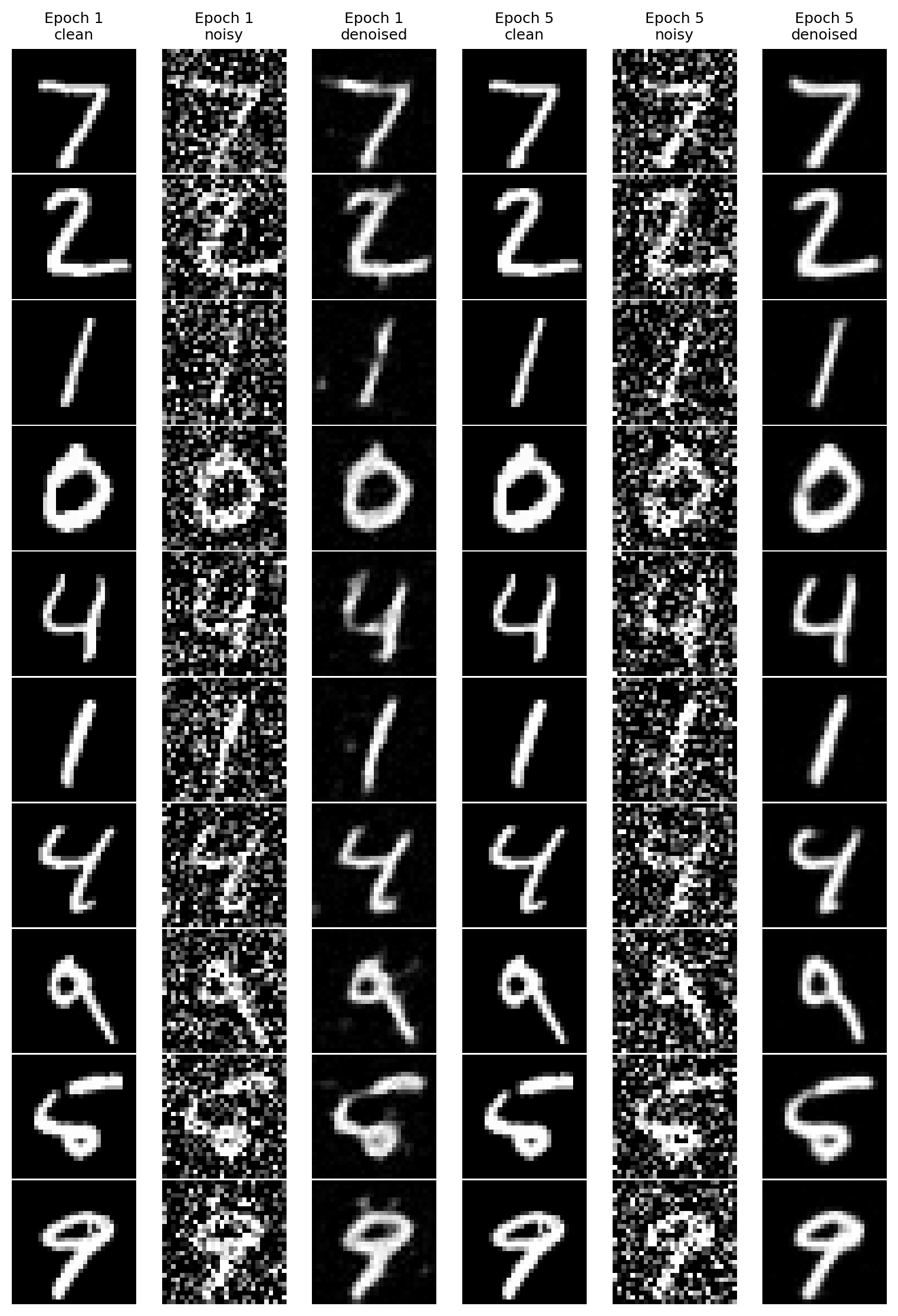
B1.2 · Training Data: (z, x) with σ=0.5 + Noising Visualization

We train on pairs z = x + σ·ε with σ=0.5 (but visualize multiple σ values to see how difficulty grows).

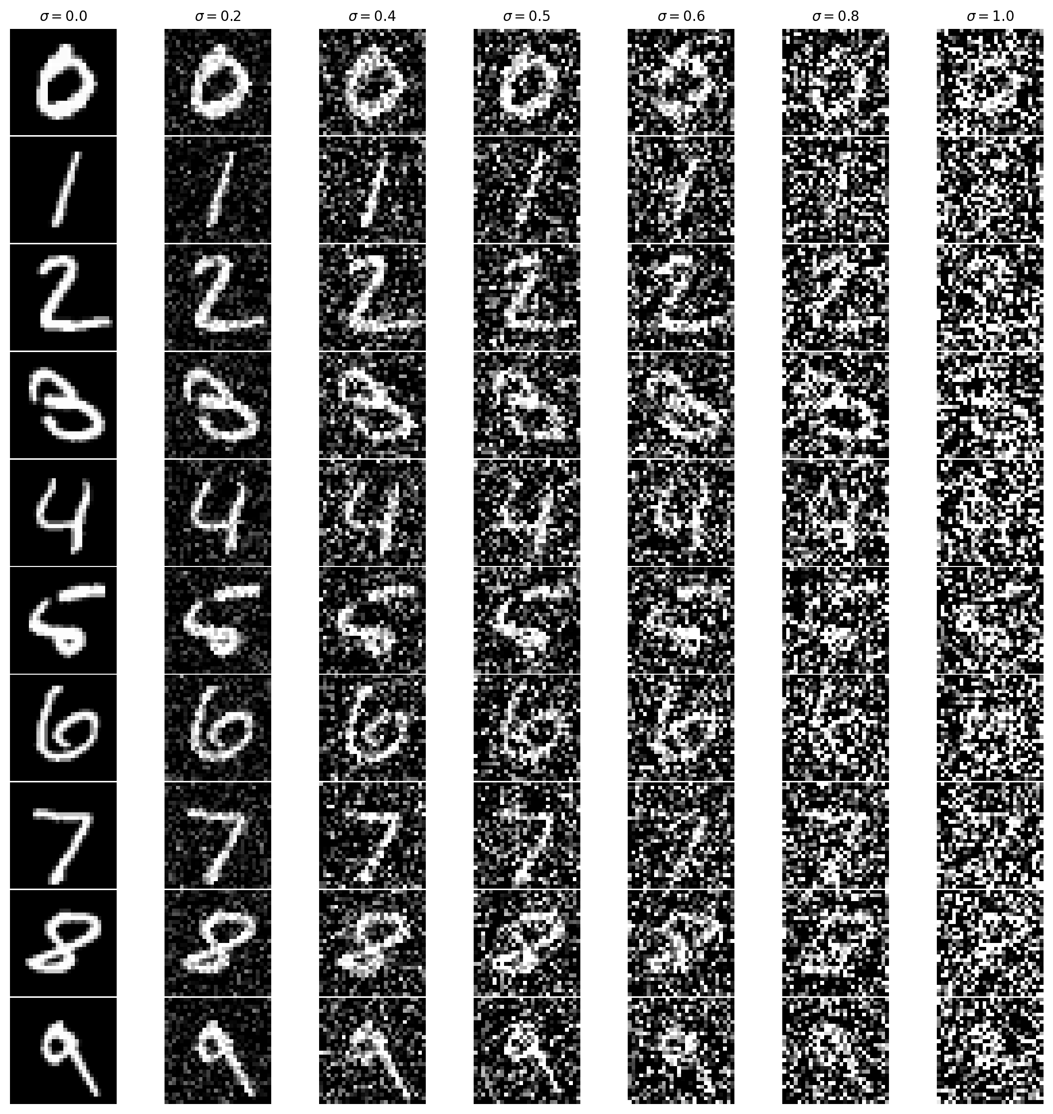
# Gaussian corruption: z = x + sigma * eps
def add_gaussian_noise(x, sigma):
    eps = torch.randn_like(x)
    z = x + sigma * eps
    return z

Walkthrough: This single function creates the entire learning problem. The model sees z (the corrupted image) and is asked to output x (the clean original). Resampling eps every iteration prevents the model from memorizing one noisy variant and forces it to learn a real denoising rule.

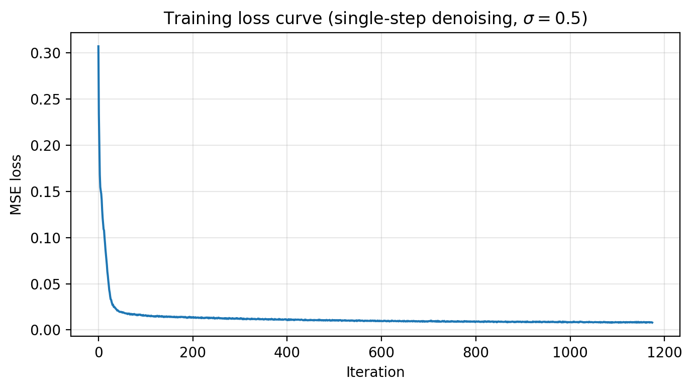
B1.2.1 · Train the Single-step Denoiser (σ=0.5)

Objective: minimize MSE ||Dθ(z) − x||². Save checkpoints after epochs 1 and 5.

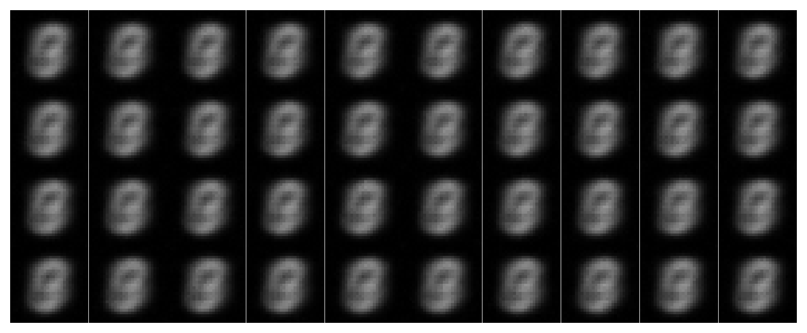
B1.2.2 · OOD Testing (σ sweep at test time)

We evaluate the σ=0.5-trained model on other σ values to see how it behaves out-of-distribution.

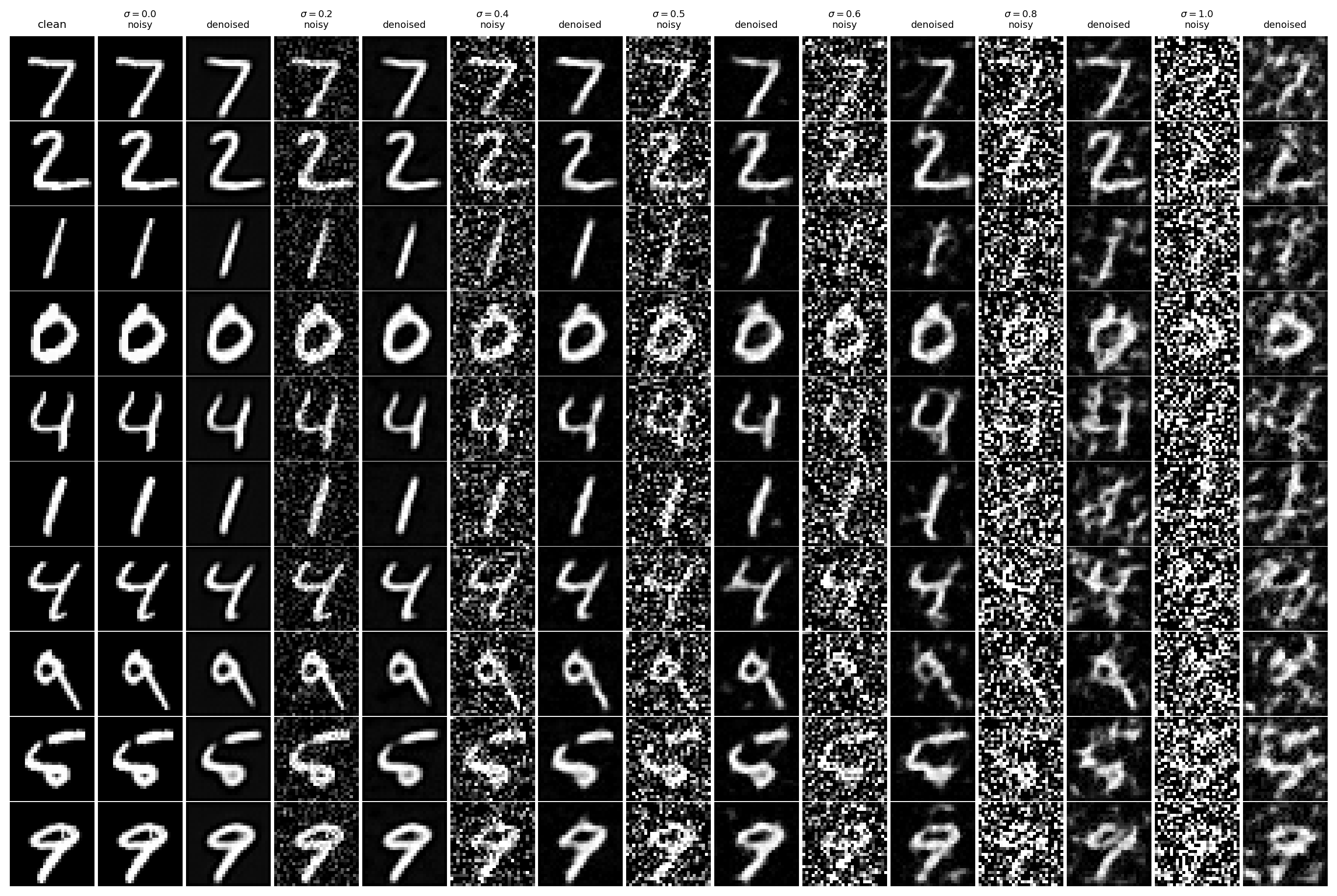
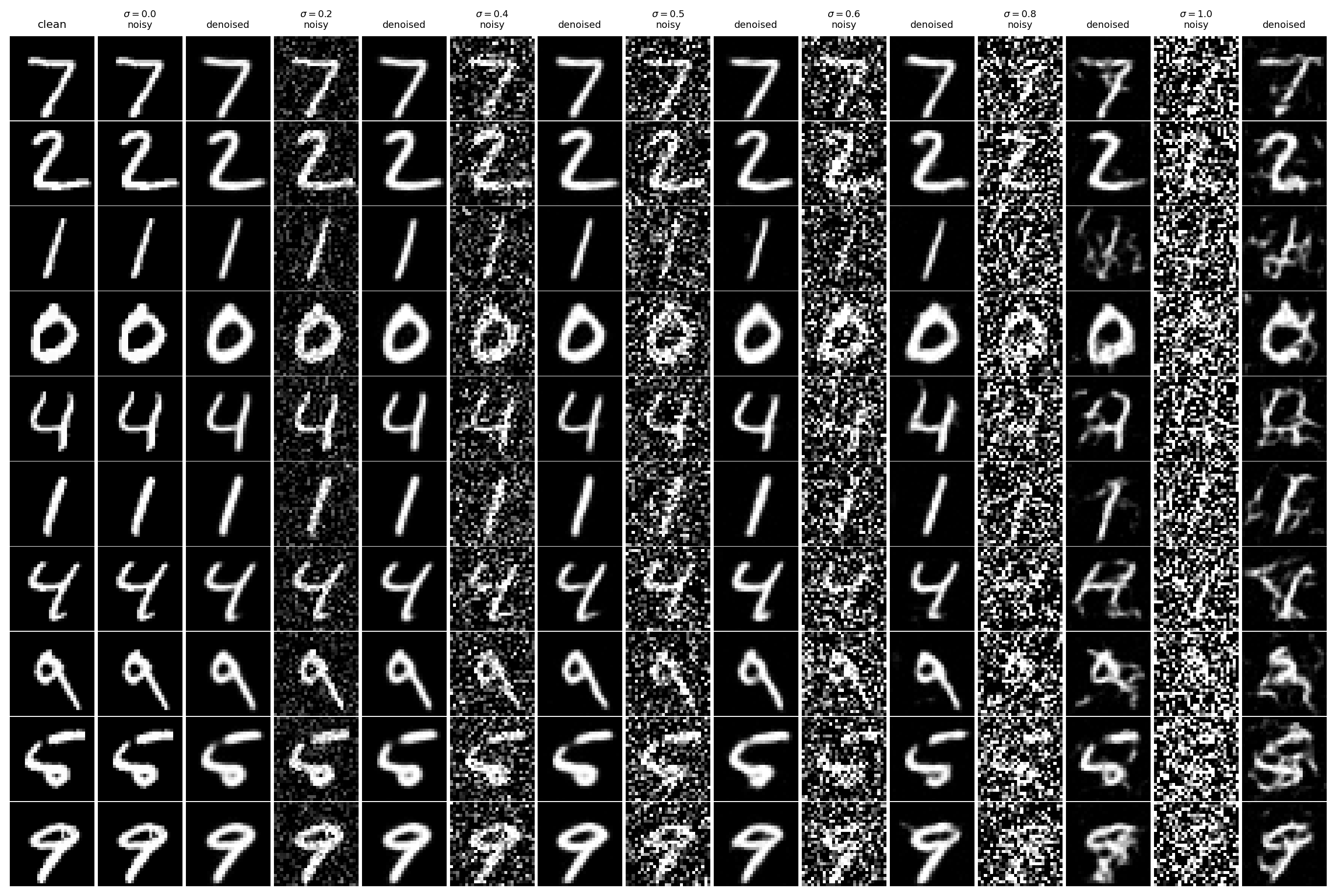
What to watch For σ < 0.5, denoising is usually easy. For σ > 0.5, the input can lose too much signal, and the model may “invent” plausible strokes to compensate.

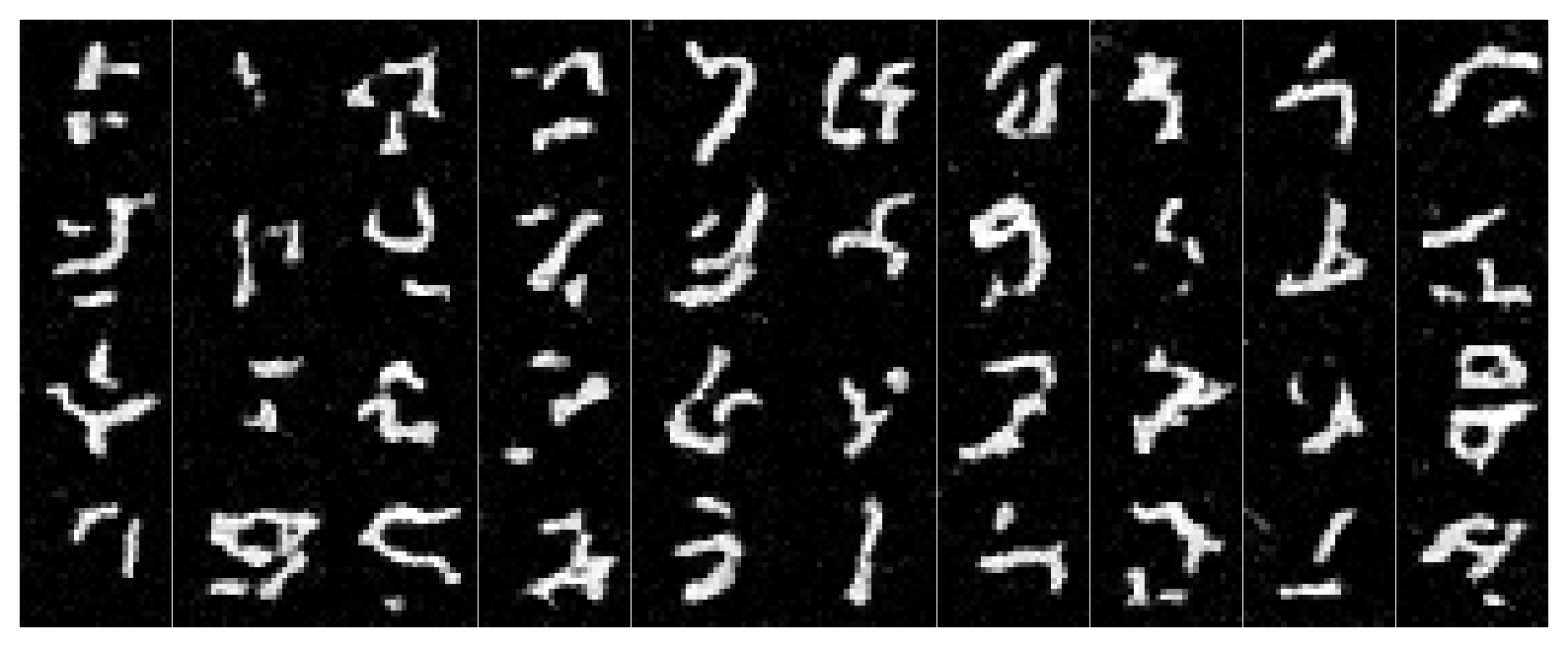
B1.2.3 · Denoising Pure Noise

Here, the input is pure noise unrelated to the target image. Under MSE, the model tends to output “average MNIST-like” structure rather than a specific digit.

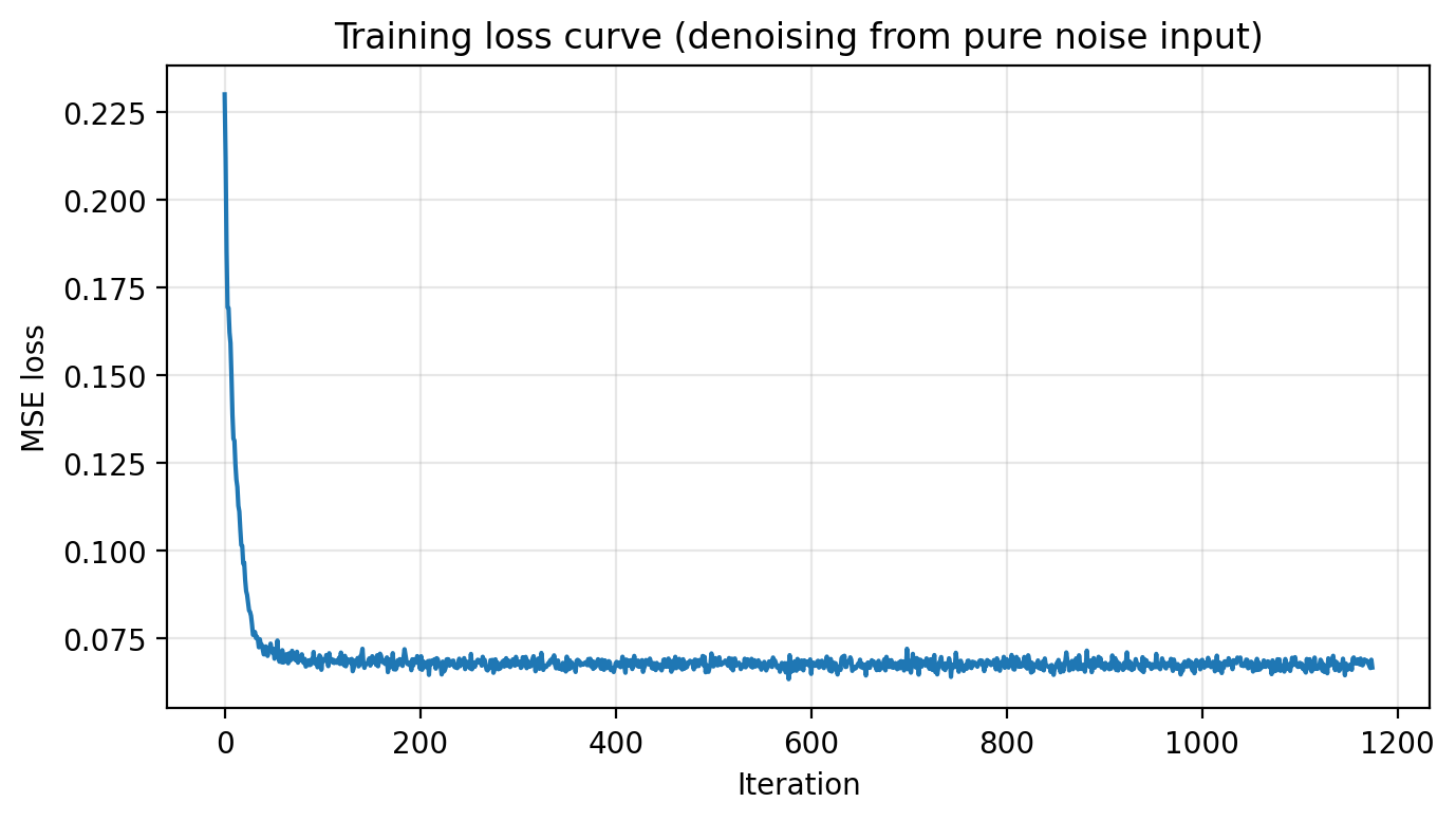
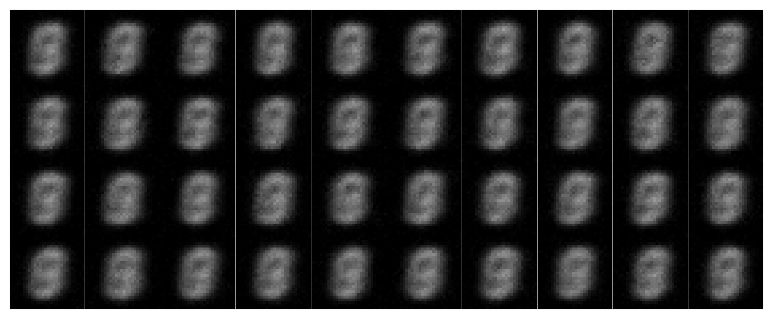
Why this happens If the input contains no information about the target, the best MSE strategy is to output something that is broadly “likely” under the dataset. That produces blurry prototypes and faint digit-like strokes: not recovery, but a learned MNIST prior leaking through.

B2 · Training a Flow Matching Model

Flow matching trains a UNet to predict the velocity that moves an interpolated point x_t = (1−t)x_0 + t x_1 from noise (x0 ~ N(0,I)) toward a data image (x1).

B2.1 · Time Conditioning (FCBlock)

We inject scalar time t ∈ [0,1] into the UNet via small MLP blocks that modulate decoder activations.

class FCBlock(nn.Module):
    def __init__(self, in_features, out_features):
        super().__init__()
        self.net = nn.Sequential(
            nn.Linear(in_features, out_features),
            nn.GELU(),
            nn.Linear(out_features, out_features),
        )
    def forward(self, x):
        return self.net(x)

Walkthrough: Time is a single number, but the UNet’s internal feature space is high-dimensional. FCBlock expands time into a rich vector so different channels can respond differently early vs late in the trajectory. This makes sampling coherent: the model can learn “big structural moves” at early t and “fine polishing moves” at late t.

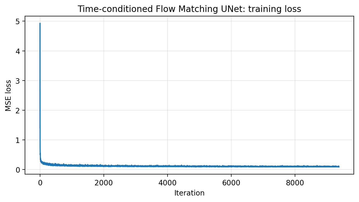
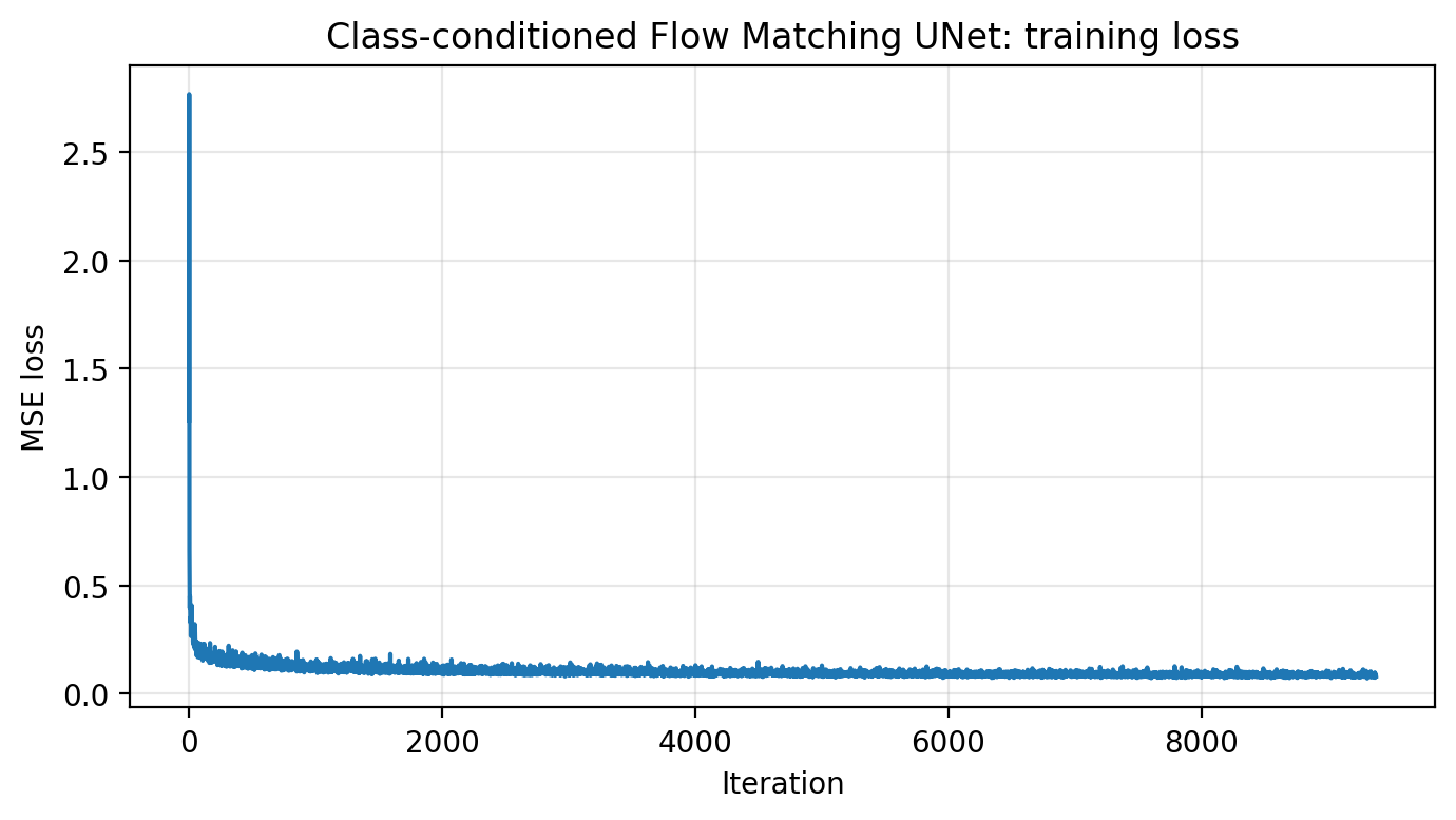
B2.2 · Train the Time-conditioned Flow Matching UNet

Loss: || (x1 − x0) − uθ(xt, t) ||². Save checkpoints after epochs 1, 5, 10.

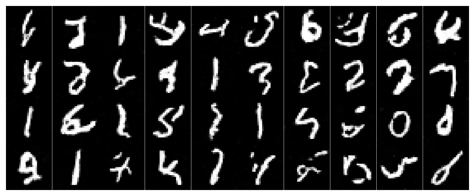
B2.3 · Sampling (Time-conditioned)

Start at x0 ~ N(0,I) and integrate forward using small steps with uθ.

B2.4 · Add Class Conditioning + Dropout (Classifier-free)

We inject a one-hot class vector c (digits 0–9), and drop it 10% of the time to learn both conditional and unconditional behaviors.

# c is one-hot (N,10). 10% of the time we drop it to 0 for classifier-free guidance later.
keep = (torch.rand(N, device=device) > 0.1).float()
c = c * keep.view(N, 1)

# Affine-ish modulation in the decoder:
unflatten = c1 * unflatten + t1
up1       = c2 * up1       + t2

Walkthrough: The class vector acts like a “destination label” for the flow field: digit-7 flows should end near digit-7 images. Dropping the class sometimes trains an unconditional flow that still produces “some MNIST digit,” which is crucial for CFG at sampling time.

B2.5 · Train the Class-conditioned UNet

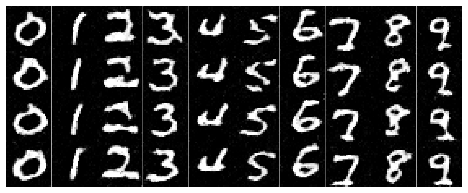
B2.6 · Sampling with Classifier-free Guidance (γ=5.0)

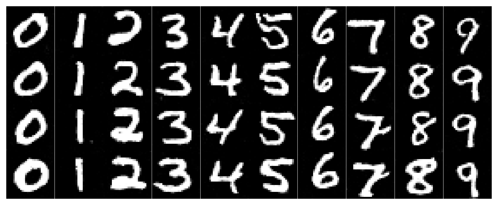
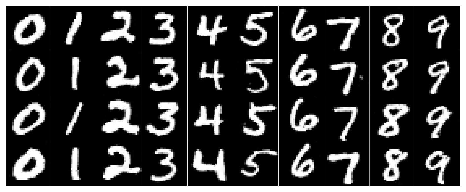
Every column corresponds to a digit 0–9. We sample conditional and unconditional flows and combine them with CFG.

# CFG for flow matching: u = u_uncond + gamma * (u_cond - u_uncond)
u_uncond = u_theta(x_t, t, c0)
u_cond   = u_theta(x_t, t, c1)
u = u_uncond + gamma * (u_cond - u_uncond)
x_t = x_t + (1/T) * u

Walkthrough: The unconditional flow says “move toward the MNIST manifold.” The conditional flow says “move toward digit k specifically.” Their difference isolates what “digit k-ness” adds. Scaling that by γ makes columns lock onto their intended class more strongly.

B · Reflection / Lessons Learned

Training the denoiser made the “magic” from Part A feel concrete: the sampling loop isn’t a spell, it’s just repeatedly applying a learned local rule. Single-step denoising is a clean supervised problem, but flow matching feels like learning a continuous transformation. Once time and class conditioning are stable, sampling becomes controllable: change the class vector, and the entire trajectory bends toward a new digit.

Implementation Notes

Unified “pitfalls” checklist (A + B)

1. Diffusion outputs (A): DeepFloyd returns (noise, variance) concatenated. If you treat variance as noise, everything looks cursed.
2. Images look washed-out: check normalization. Many pipelines use [-1,1] internally and need mapping to [0,1] for display.
3. CFG produces artifacts: lower scale, or use fewer steps. Too strong guidance can “force” texture hallucinations.
4. Inpainting won’t respect the background: ensure you overwrite the unmasked region every step, using the correctly noised original.
5. Anagrams don’t read both ways: try more steps or choose prompts with compatible visual geometry (two concepts that can share shapes).
6. Scheduler stepping per iteration: your LR collapses too fast, model stops learning.
7. Condition shapes: ensure time is (N,1) before FCBlock, and reshape outputs to (N,C,1,1) for broadcasting.
8. CFG formula: use u = u_uncond + γ (u_cond − u_uncond) (difference, not sum).
9. Clamping: clamp only for visualization; clamping during training can hide error signals.